
EOQ Model versus (Q,r) Model: Case Study of a Company's Inventory in Londrina, Paraná, Brazil

DOI 10.5433/1679-0375.2024.v45.51741
Citation Semin., Ciênc. Exatas Tecnol. 2024, v. 45: e51741
Received: 6 November 2024 Received in revised for: 16 December 2024 Accepted: 26 December 2024 Available online: 28 December 2024
Abstract:
This article presents mathematical and statistical methods applicable to inventory management. Inventory analysis using ABC curves is used to identify priority items, the most expensive items, and those with the highest turnover (demand). Based on this information, it is possible to determine, through inventory control models, the optimal order quantity and frequency that minimize the total storage costs of these items. Using the Economic Order Quantity (EOQ) model and the \((Q, r)\) model, inventory control models, the minimization of a company’s inventory costs in Londrina, Paraná, Brazil was simulated. The comparison of the results provided by the models was discussed. Specifically, it was observed that for some inventory items, it would theoretically be possible to achieve savings margins of over 50% on inventory expenses for this company.
Keywords: inventory management, ABC curves, EOQ model, \((Q, r)\) model, cost minimization
Introduction
Difficulties and problems are common in any business environment. In inventory management, we identify problems related to the control and organization of materials. There is a great need to stock materials for production, but stocking materials has a cost. Problems with inventory organization and sizing have important repercussions within a company. According to Ching, 2009, inventory must be efficient, as it is integrated into the company’s production chain.
Materials management in a company is an activity whose main objective is to meet the needs and expectations of customers. According to Gonçalves, 2013, in the traditional format, materials management aims to harmonize the interests between supply needs and the optimization of companies’ financial and operational resources. Well-structured materials management allows for competitive advantages to be obtained through cost reduction, reduced investment in inventory, improvements in purchasing conditions through favorable negotiations with suppliers, and customer and consumer satisfaction with the products offered by the company.
In this context, our study aims to use mathematical models and numerical simulations to improve the performance of the inventory of a company in the city of Londrina, Paraná, Brazil, leaving it, as far as possible, in its best organizational, functional, and profitable form.
The company studied needs to improve its inventory management. Among the main problems observed, we can mention the discrepancy between the actual physical inventory and the calculated accounting inventory, and the large opportunity purchases of inventory items. Opportunity purchases occur when an inventory item has a falling price, and large volumes of these inventory items are acquired. Such purchases, usually on impulse, do not consider the costs of storage for long periods and the storage capacity (physical space). In such situations, the solution is usually to store excess material in containers or rent spaces outside the company.
To minimize the inventory costs of this company in Londrina, Paraná, Brazil, we have used mathematical models and numerical simulations. The mathematical models used in this study to optimize the order quantities in stock are the Economic Order Quantity (EOQ) model (Agarwal, 2014; Battini et al., 2014; Nobil et al., 2020; Çalışkan, 2021; Oliveira et al., 2022; Alnahhal et al., 2024) and the \((Q,r)\) model (Namit & Chen, 1999; Pan et al., 2004; Mattsson, 2007; Kouki et al., 2015; Parviz et al., 2015; Braglia et al., 2019; Pilati et al., 2024). Through these inventory control and optimization models, it is possible to obtain the optimal level of quantity and frequency orders for each inventory item, which minimizes the company’s total inventory storage costs.
Materials and methods
There are numerous mathematical models and efficient tools that help optimize and resolve inventory problems. In this paper, we will not study models focused on organizing or distributing items within the inventory. Such models aim to facilitate access to items and minimize the time and costs generated by the movement of materials within the inventory, and from the inventory to production. In this article, we will study mathematical models and tools to minimize storage costs for the inventory of the company studied (Waters‐Fuller, 1995; Tripathi, 2013; Riza et al., 2018; Adegbola et al., 2024).
The mathematical tools in this study are designed to determine:
the optimal order quantities of each inventory item,
the optimal reorder times for each inventory item, and
the minimum (optimal) costs for inventory management.
Note that such control techniques and methodologies can be applied to all inventory items; on the other hand, not all stored items deserve the same attention from management or need to maintain the same availability in inventory (Ching, 2009).
ABC curves
The ABC curve is based on the concept of the Pareto rule, in which not all items have the same importance and attention should be given to the most significant ones (Chen et al., 1994; Müller et al., 2014; Parviz et al., 2015; Wuni, 2022).
The ABC curve model classifies inventory items into 3 categories, related to the monetary values of each inventory item. The monetary value is the result of multiplying the total demand for this item in a period by its unit price, representing its effective participation in the monetary dynamics of the inventory. Thus, each inventory item must be classified according to its monetary value, so that an appropriate inventory policy can be established. The ABC curve method and the Pareto rule allow this policy to be carried out through the classification of priority items.
Through this mathematical modeling, the representativeness of each inventory item is given by its monetary value. Thus, by listing the monetary values of each item in descending order, it is possible to calculate the relative percentage of participation of each item concerning the total inventory cost, given by the sum of all monetary values. Table 1 exemplifies such procedures. Note that Item 1 represents 3% of the monetary value of the entire inventory and that items 1, 2, and 3 together represent 7.75%.
| Item name | Annual demand | Unit price | Monetary value | % Relative | % Accumulated |
|---|---|---|---|---|---|
| Item 1 | 12,000 | R$ 10.00 | R$ 120,000.00 | 3.00% | 3.00% |
| Item 2 | 6,667 | R$ 15.00 | R$ 100,005.00 | 2.50% | 5.50% |
| Item 3 | 10,000 | R$ 9.00 | R$ 90,000.00 | 2.25% | 7.75% |
| . | . | . | . | . | . |
| . | . | . | . | . | . |
| . | . | . | . | . | 99.50% |
| . | . | . | . | 0.03% | 99.80% |
| Item n | . | . | . | 0.02% | 100.00% |
| Total | R$ 4,000,000.00 | 100.00% |
In ABC classification, class A items have the highest priority. The following proportions are typically adopted for each class interval:
Class A: Priority items given by the Pareto rule. These are the items with the highest monetary value, the first items of Table 1, and which account for up to 80% of the accumulated percentage of participation.
Class B: Intermediate items. These are the items that account for 80% to 95% of the accumulated percentage of participation.
Class C: Low-priority items. These are the last items of Table 1, those with low monetary value that account for 95% to 100% of the accumulated percentage of participation.
The proportions assigned to each ABC class range may vary from case to case. A recurring feature of the ABC curve is that a small portion of the items are class A, while the vast majority of the items are class C. In general, approximately 20% of the items are responsible for 80% of the accumulated monetary values of all items, this is Pareto’s 80 \(\times\) 20 rule.
EOQ model
In general, in any type of inventory, regardless of the material contained in it, the associated costs are basically related to (Waters‐Fuller, 1995; Tripathi, 2013; Riza et al., 2018; Adegbola et al., 2024):
maintenance costs,
order costs, and
shortage costs.
To simplify, assuming that there are no item shortages, the total cost generated by inventories would is the sum of maintenance and order costs. The EOQ model takes these costs into account. A critical issue is balancing these costs, as they have different behaviors. Note that the larger the quantities stored, the more space these products will take up in the inventory and the higher the maintenance costs will be. On the other hand, the larger the purchase quantities, the smaller the order quantities will be, and consequently, the lower the ordering costs (Agarwal, 2014; Battini et al., 2014; Nobil et al., 2020; Çalışkan, 2021; Oliveira et al., 2022; Alnahhal et al., 2024). The curves in Figure 1 illustrate these inventory costs.
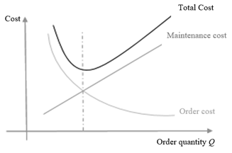
Adapted from “Economic order quantity model: A review” by Agarwal, S., 2014, VSRD International Journal of Mechanical, Civil, Automobile and Production Engineering, 4(12), 233–236.
Note in Figure 1 that the total cost function has the shape of an upward concave curve, meaning there is a minimum value for the total inventory cost. It can be seen (as we will see later) that this minimum occurs precisely at the intersection of the curves for maintenance and order costs. Note that the description above becomes more complex if we consider item shortage costs, inflation, and other costs.
To aid understanding, it is important to define and differentiate the meaning of item demand \(D\) and order quantity \(Q\). The demand \(D\) for an inventory item is the quantity (annual, for example) that was requested of that specific item by the production line, while the order quantity \(Q\) is the quantity that will be purchased of that item at each replenishment. Simply put, the annual demand \(D\) for an item can be met through \(n\) purchases during the year, with order quantity \(Q\).
The Economic Order Quantity (EOQ) model is a basic inventory control model. It allows determining the optimal order quantity \(Q\) for inventory items, considering the minimization of total inventory costs \(C_T\). In the EOQ model (Hillier & Lieberman, 2013; Stadtler et al., 2014), the total inventory cost is a function of the order quantity \(Q\), namely:
\[ C_T = f(Q) = \frac{Q}{2} C_m + \frac{D}{Q} C_p + D P,\]
where \(Q\) is the order quantity of the item, \(D\) is the annual demand quantity of the item, \(P\) is the purchase unit price of the item, \(C_m\) is the annual maintenance unit cost, also known as the carrying cost or storage cost of the item, and \(C_p\) is the order unit cost, also known as the setup cost of the item.
Note that the first term, in equation (1), maintenance costs, are costs directly proportional to the quantity stored (storage costs, insurance costs, handling costs, obsolescence costs, and others). The second term, order costs, are costs inversely proportional to the quantity stored (labor costs, order transportation costs, product receipt costs, quality control costs, and others). Finally, the third term, acquisition costs, corresponds to the acquisition costs of the items in inventory.
As we can see in Figure 1, the total cost function \(f(Q)\) of the inventory is concave upwards. To find the value of order quantity \(Q\) that minimizes the total cost \(C_T\), one must differentiate \(f(Q)\) with respect to the parameter \(Q\) and set the derivative equal to zero.
The value of the optimal order quantity \(Q^*\) of the EOQ model is given by Hillier & Lieberman, 2013; Stadtler et al., 2014
\[ {Q^*} = \sqrt{\frac{2 D C_p}{C_m}}.\]
Note that by equating the maintenance and order costs, the first and second terms of equation (1), we also obtain the result given in equation (2), that is, the minimum cost presented in Figure 1 occurs at the intersection of maintenance and order cost curves.
\((Q, r)\) Model with shortage cost
In the EOQ model, demand and consumption rate are known quantities, with the consumption rate being considered constant. On the other hand, the \((Q, r)\) model is a stochastic model, that is, it is a model that was developed to analyze inventory systems in which there are considerable uncertainties about future demands (Namit & Chen, 1999; Pan et al., 2004; Mattsson, 2007; Kouki et al., 2015; Parviz et al., 2015; Braglia et al., 2019; Pilati et al., 2024).
In this model, inventory must have a continuous review system, with the inventory level being monitored continuously so that it is possible to know the exact quantity of each item at the present time (Hillier & Lieberman, 2013).
The \((Q, r)\) model is based on determining two critical quantities: \(r =\) reorder point and \(Q =\) order quantity of the item. The inventory policy of the \((Q, r)\) model is simple, that is, whenever the product inventory level drops to \(r\) units, an order for \(Q\) additional units must be placed to resupply the inventory. Please note that if there is an order failure, then a shortage of items and consequently a shortage costs may occur.
The value of the optimal order quantity \(Q^*\) of the \((Q, r)\) model with shortage costs is given by Hillier & Lieberman, 2013:
\[ {Q^*} = \sqrt{\frac{2 D C_p}{C_m}} \sqrt{\frac{C_f + C_m}{C_f}},\]
where \(C_f\) is the shortage cost, and the other quantities are already described in equation (1). Note that when an item is out of stock, a shortage cost \(C_f\) is incurred. The \((Q, r)\) model aims to avoid shortages or a lack of items in stock.
To define the reorder point \(r\) in a company’s inventory, an analysis of the desired service quality level for customers must be conducted. In general, the most common choice is to define a variable \(0 \leq L \leq 1\), which represents the desired probability that there will be no shortage of inventory during the lead time from order to delivery. In other words, the demand for the production line during the lead time is expected to be less than the quantity in stock at the time of order, with probability \(L\).
To implement this mathematical modeling, we must choose a probabilistic distribution for the random variable \(C_i\), which is the consumption during lead-time periods. Suppose the lead-time is 5 days, then \(C_1\) is what was consumed in the last 5 days of lead-time, \(C_2\) is what was consumed in the penultimate 15 days of lead-time before \(C_1\), and so on until \(C_n\). From these \(C_i\) we must fit a probabilistic distribution (Gaussian, Poisson, Gamma, etc.). We choose to fit a symmetric Gaussian probabilistic distribution with mean and variance given by equations (4) and (5):
\[ \mu^* = \hat{C} = \frac{\sum_{i=1}^{n} C_i}{n},\]
\[ \sigma^{2*} = \frac{\sum_{i=1}^{n} (C_i - \hat{C})^2}{n-1}.\]
We can then calculate the value of \(r\) by transforming the distribution of \(C_i\) to a symmetric Centered Normal distribution \(Z\) with mean \(\hat{C} = 0\) and variance \(\sigma^{2*} = 1\). According to Morettin & Bussab, 2013, from this new distribution, you can obtain \(r\) as:
\[ r = \mu^* + Z_L \sqrt{\sigma^{2*}},\]
where \(Z_L\) is the integrated value corresponding to the result of the accumulated symmetric Centered Normal distribution function up to probability \(L\), that is:
\[ Z_L = \frac{1}{\sqrt{2\pi}} \int_{-\infty}^{L} e^{-\frac{x^2}{2}} \, dx,\]
whose values are tabulated in Morettin & Bussab (, p. 519).
Determination of \(C_m\) and \(C_p\)
To apply the EOQ and \((Q, r)\) models to the optimization of the company’s inventory, we need to know the values of the storage unit cost parameters \(C_m\) and order unit cost parameter \(C_p\). Note that the company does not have the storage and order costs for each item in the inventory; it has the costs of all items, so we cannot individually calculate the quantities \(C_m\) and \(C_p\) for each item in the inventory. We will consider the average value of \(C_m\) and \(C_p\) for all items.
Let the annual storage costs, denoted by \(C_M\), be the sum of inventory personnel costs (payroll and labor charges), inventory maintenance costs (rent, taxes, insurance, maintenance, ...), office costs (paper, materials, printers, ...), handling costs (forklifts, fuel, ...), inventory general costs (water, electricity, telephone, ...), among others.
Let the annual order costs, denoted by \(C_P\), be the sum of order personnel costs (payroll and labor charges), office costs (paper, materials, printers, ...), transportation costs (fuel, freight, tolls, ...), order general costs (water, electricity, telephone, ...), among others.
Once the total annual storage costs \(C_M\) and the total order costs \(C_P\) have been quantified, we can calculate the unit quantities \(C_m\) and \(C_p\). Modeling the mathematical calculation of these quantities, we propose that they be given by the equations (8) and (9):
\[ C_m = \frac{C_M}{A_{t}},\]
\[ C_p = \frac{C_P}{E_{t}},\]
where \(A_t\) is the sum of all areas of the movement graphs of all class A items, that is, it is the sum of all units of each item A in stock during the year, while \(E_t\) is the order sum of all items A in stock during the year.
Results
The data and results presented below refer to the minimization of inventory costs for a company in Londrina, Paraná, Brazil. The historical records of inputs (entry) and outputs (exit) of all their inventory items from 2009 to 2016 were provided. To illustrate the size of this company’s inventory, in 2016, there was movement of 569 different items, 2,948 purchase orders, and 147 situations of stockout situations.
Stock movement data
Consider Table 2, which shows a hypothetical movement of products in a company’s inventory. It provides the type/name of the item; the movement type (\(E =\) entry or \(S =\) exit); the date of the movement; the quantity (in units) and (in kg), positive if entered, negative if left.
| Type/Name | Movement type | Date movement | Quantity (units) | Quantity (Kg) |
|---|---|---|---|---|
| Item 1 | E | 10/01/2011 | 200 | 22.8 |
| Item 1 | S | 24/09/2011 | -300 | -34.2 |
| Item 2 | E | 10/01/2011 | 734 | 88.1 |
| Item 2 | E | 31/03/2011 | 3352 | 402.2 |
| Item 3 | E | 17/08/2011 | 1500 | 265.5 |
| Item 3 | E | 20/10/2011 | 300 | 531.0 |
| Item 3 | S | 30/08/2011 | -692 | -122.5 |
| Item 3 | S | 31/08/2011 | -682 | -120.7 |
| Item 4 | E | 14/01/2011 | 400 | 12.0 |
| Item 4 | S | 05/01/2011 | -60 | -1.8 |
Assume that price/kg of the inventory items are known, then, from the annual quantities moved of each item in the inventory, we obtain the monetary value classification of the items in that year and, consequently, the ABC curve of the inventory.
Items classified as A represent 80% of the monetary values of the inventory, while items classified as B and C represent the remaining 20%. Normally, items classified as A are few and the vast majority are those classified as B and C, this is the Pareto Principle. In this context, to optimize the inventory, we will consider only items classified as A. This procedure is useful when the inventory has hundreds of different items stored.
In the case study considered, the result obtained for the classification of ABC items in the company’s inventory showed that 97 items were class A, 116 items were class B, and 356 items were class C. Note that 97 class A items, from a total of 569 items, correspond to 17% of the inventory items, that is, only 17% of all items were responsible in 2016 for 80% of the financial movement in the company’s inventory.
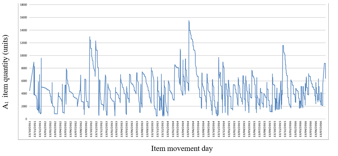
Therefore, having class A items in stock, it is possible to analyze the graphs of the movement of these items in recent years to observe whether they have stable turnover frequencies, whether the movement is periodic, in which period of the year do the biggest purchases occur and what the general movement behavior of these items is. This information allows us to analyze whether the stored quantity of this specific item is negatively impacting inventory costs. Below we present three different dynamics of movement of inventory items of a company located in Londrina, Paraná, Brazil.
Figure 2 shows the movement of one item in the company’s inventory, called item \(A_1\), which presents a certain homogeneity in its movements (oscillations), without many large peaks and with periodic movements. This type of movement is the situation desired by the \((Q, r)\) and EOQ models. On the other hand, the models can propose the order quantity \(Q\) and the reorder point \(r\) that minimize the costs of this inventory.
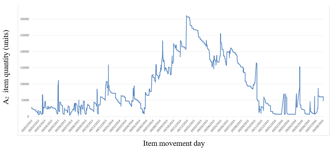
In Figure 3, we observe the movement graph of an inventory item, called item \(A_2\), which presents an accumulation of entries (purchases) in the period between June 2014 and December 2014. Consequently, during this period, large quantities of this item increased inventory costs, and even with an excess of this item in inventory, purchases still occurred, probably opportunity purchases, such as the one that occurred in December 2014. In such circumstances, the EOQ and \((Q, r)\) models can propose a more economical inventory management.
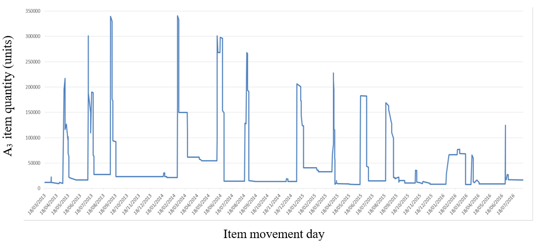
There are also cases of items with movement such as that shown in Figure 4, where we observe that an item in the inventory, called item \(A_3\), is purchased and immediately used. This "Just In Time" type of movement means that the items remain in the inventory for a short time, which is good. Just In Time movement is a model that aims for minimum inventory use, which is an optimal situation, by definition. In this case, the EOQ and \((Q, r)\) models cannot improve the inventory management of these items. For the movement of items using the “Just In Time” methodology to be effective, a short reorder time is necessary, otherwise, there will be high shortage costs (Waters‐Fuller, 1995).
Applications to EOQ and \((Q, r)\) models
We will apply the EOQ and \((Q,r)\) models to the same A-classification item, in order to compare the results obtained. As one of the fundamental assumptions of the EOQ model is that the movement rate of inventory items is carried out continuously and constantly, then we must select an inventory item that has movement with these characteristics, so that we can compare the models. This selected item will be called item \(A_4\).
Figure 5 shows the movement of inputs and outputs of an inventory item during the year 2016. Note that in 2016 the movement of this item presents two large purchases of approximately 9500 units and several other smaller purchases of up to 2000 units. The first question that arises is whether these purchase sizes are economically efficient. This answer can be obtained from the analysis carried out by the inventory management models.
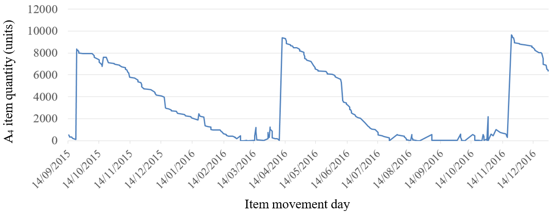
Next, we will analyze some characteristics of this item’s movement. First, we must verify that the movement of the item shown in Figure 5 has a constant and continuous consumption rate over time, as required by the EOQ model. From the data in Figure 5, we have that during 2016, 25,550 units of this item were purchased (peaks in Figure 5. Figure 5 also provides us with the consumption of this item during 2016. Thus, starting from 25,550 units of this item, Figure 6 shows the consumption rate of this item throughout 2016. Note that the consumption rate of this item remained practically constant and continuous during 2016. So, for an annual purchase of 25,550 units, the daily consumption rate of this item is approximately constant at 70 units per day.
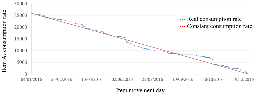
Note that the consumption rate of the item shown in Figure 6 presents the characteristics required by the EOQ model. Thus, the A-classification inventory item, which presents the movement shown in Figure 5, will be designated as item \(A_4\), which will be used in the cost comparison between the EOQ and \((Q,r)\) models.
Inventory cost minimization - EOQ model
Let us apply the EOQ model to minimize the storage costs of item \(A_4\) whose movement is given in Figures 5 and 6. From the inventory information of the company in question, we have calculated the following parameters, presented in Table 3.
| D | Cm | Cp |
|---|---|---|
| 25,550 units | R$ 1.00 | R$ 50.00 |
Substituting these parameters into equation (2), we obtain \(Q_{\text{EOQ}}^* \sim 1600 \text{ units}\).
Therefore, to meet the daily demand for item \(A_4\) in 2016, the ideal purchase size that would minimize inventory costs would be approximately 1600 units.
Regarding the reorder point \(r\) for item \(A_4\) in 2016, since the consumption rate is 70 units per day and the delivery time (lead time) of item \(A_4\) is 14 days, then from the EOQ model:
\[ r_{\text{EOQ}} ={70 \times 14} = 980 \text{ units.}\]
Finally, let us calculate the savings in storage costs due to the EOQ model proposal, considering only item A4 of the inventory. To do this, we need to calculate the storage costs and order costs of item \(A_4\), as modeled in equation (1).
Note that in equation (1), the quantity \(Q/2\) represents the average stock in a period, while the quantity \(D/Q\) is the total number of orders in the same period. For item \(A_4\), during 2016, this information can be extracted from Figure 5. Table 4 shows these results.
| Average stock (units) | Total number of orders | |
|---|---|---|
| Data | 2580 | 24 |
Considering maintenance and ordering costs, from equation (1) it follows that the realized storage cost of item \(A_4\) during 2016 was:
\[ \text{Realized storage cost} = {2580 \times 1 + 24 \times 50} = \text{R\$ } 3780.00.\]
Now let us calculate how much would have been spent if the company had made periodic purchases of 1600 units of item \(A_4\), as proposed by the EOQ model. From equation (1) it follows that:
\[ \text{EOQ model predicted storage cost} = {\frac{1600}{2} \times 1 + \frac{25550}{1600} \times 50} \sim \text{R\$ } 1600.00.\]
Finally, note that by managing the company’s inventory using the EOQ model, considering only inventory item \(A_4\), the company could have theoretically saved R$ 2180.00.
Inventory cost minimization - \((Q, r)\) model
The parameters estimated or provided by the company for the calculations for the \((Q, r)\) model are presented in Table 5.
| D | Cm | Cp | C_f | Lead time |
|---|---|---|---|---|
| 25,550 units | R$ 1.00 | R$ 50.00 | R$ 4.00 | 14 days |
Note that the lead time for item \(A_4\) is known, 14 days, and \(C_f\) is the cost per stockout provided by the company, which occurs when an item is out of stock. Substituting these values into equation (3), it follows that the optimal order quantity, given by the \((Q, r)\) model for item \(A_4\), is \(Q_{(Q,r)}^* \sim 1800 \text{ units}\).
To determine the reorder point given by the \((Q, r)\) model, it is necessary to extract some more information about item \(A_4\), such as the mean \(\mu^*\) and the variability \({\sigma^2}^*\) of the consumption of item \(A_4\) in 2016, as shown in equations (4) and (5). We chose a Gaussian distribution to calculate these quantities. We also chose \(L = 0.75\), the probability desired by management so that stockouts do not occur. These data are presented in Table 6.
| L | \(\mu^*\) | \(\sqrt{{\sigma^2}^*}\) |
|---|---|---|
| 0.75 | 981.75 | 721.21 |
From the data in Table 6 and equations (6) and (7), we obtain the reorder point of the \((Q, r)\) model (Morettin & Bussab, , p. 519)
\[\nonumber {r_{(Q, r)} \sim 1400 \ \text{units}}.\]
Table 7 compares the results obtained by the \((Q, r)\) model, considering a 75% probability that no shortage will occur, with the results obtained by the EOQ model.
| Model | Ideal purchase (units) | Reorder point (units) |
|---|---|---|
| EOQ | 1600 | 980 |
| \((Q, r)\) | 1800 | 1400 |
Note that the result obtained for the optimal order quantity by the \((Q, r)\) model is greater than that obtained for the EOQ model. Similarly, the reorder point obtained by the \((Q, r)\) model is also greater than the EOQ reorder point. The word “caution” explains these results. Unlike the EOQ model, the \((Q, r)\) model takes into account the costs of shortages and the probability of stockouts, which provides greater assurance in cases of emergencies and unpredictability.
In general, for stable economies where future demands and expenses are predictable, the EOQ model is a good choice to provide the quantities to be purchased, as it minimizes total storage costs. On the other hand, in Brazil where the company is located, the economy is unstable (fluctuations in exchange rates, interest rates, taxes, etc.), which generates large fluctuations in the movement of inventory items, so that the movement of inventory items is not constant and continuous over time. In this context, it is recommended for the company to use the \((Q,r)\) model to manage its inventory.
Finally, let us see how much would have been spent on storage if we had purchased quantities of 1800 units of item \(A_4\), as proposed by the \((Q, r)\) model. From equation (1):
\[ \text{(Q, r) model predicted storage cost} = {\frac{1800}{2} \times 1 + \frac{25550}{1800} \times 50} \sim \text{R\$} 1610.00.\]
Note the small difference between the storage costs predicted by the EOQ model, equation (12), and by the \((Q, r)\) model, equation (13).
Models summary
Table [tab:8] presents a summary of the results obtained in the inventory management of this company through the EOQ and \((Q,r)\) models of \(A_4\) inventory item.
| Item | EOQ Model | \((Q,r)\) Model |
|---|---|---|
| Ideal purchase size \(Q^*\) | 1600 units | 1800 units |
| Reorder point \(r\) | 980 units | 1400 units |
| Realized storage cost | R$ 3780.00 | - |
| Proposed storage cost | R$ 1600.00 | R$ 1610.00 |
| Saved storage cost | R$ 2180.00 | - |
Conclusions
This paper demonstrates the procedures for optimizing a company’s inventory. In the case study of item, designated as item \(A_4\), of a company in Londrina, Paraná, Brazil, inventory management models predicted savings of over 50% in inventory costs. The application of inventory management models, specifically the EOQ and \((Q,r)\) models, revealed significant cost savings in inventory operations.
We emphasize that maintenance and ordering costs do not necessarily decrease with inventory reduction, as predicted in the EOQ and \((Q,r)\) models. For example, the insurance paid by the company will probably not decrease with the reduction of inventory, since inventory is only one part of the company.
Typically, in inventory management, it is observed that inventory movements are random, and purchases are oversized, mainly due to opportunity purchases. In this context, if future demands are predictable, the EOQ model is a good choice to provide the quantities to be purchased, those that will minimize total storage costs.
On the other hand, we found that the savings obtained with inventory management conducted by the EOQ and \((Q,r)\) models generate very similar results. Therefore, in the context of an unstable economy, in which there are fluctuations in exchange rates, interest rates, taxes, etc., it is more viable to use the \((Q,r)\) model, which will provide a greater guarantee for inventory management.
Author contributions
C. K. Oliveira participated in: Programs, Validation, Visualization, and Writing (preparation of the original draft). P. L. Natti participated in: Conceptualization, Project Management, Programs, Supervision, Validation, Visualization, and Writing (revision and editing). E. R. T. Natti participated in: Conceptualization, revision and editing. E. R. Cirilo participated in: Project Management, Validation, Visualization, and Writing (revision and editing). N. M. L. Romeiro participated in: Supervision and Writing (revision and editing).
Conflicts of interest
The authors declare no conflict of interest.
References
Agarwal, S. (2014). Economic order quantity model: a review. 4(12), 233--236.
Braglia, M., Castellano, D., Marrazzini, L. & Song, D. (2019). A continuous review, $(Q, r)$ inventory model for a deteriorating item with random demand and positive lead time. 102--121. https://doi.org/10.1016/j.cor.2019.04.019
Chen, Y.-S., Chong, P. P. & Tong, M. Y. (1994). Mathematical and computer modelling of the Pareto principle. 19(9), 61--80. https://doi.org/10.1016/0895-7177(94)90041-8
Ching, H. Y. (2009). Gestão de estoque na cadeia de logística integrada: supply chain. Editora Atlas.
Gonçalves, P. S. (2013). Administração de materiais. Elsevier.
Kouki, C., Jemaï, Z. & Minner, S. (2015). A lost sales (r, Q) inventory control model for perishables with fixed lifetime and lead time. 143--157. https://doi.org/10.1016/j.ijpe.2015.06.010
Hillier, F. S. & Lieberman, G. J. (2013). Introdução à pesquisa operacional. AMGH Ed.
Oliveira, C. K., Natti, P. L., Cirilo, E. R., Romeiro, N. M. L. & Natti, E. R. T. (2022). Gestão de estoques: uma aplicação do modelo do Lote Econômico de Compra. Atena Editora. 46--60. https://doi.org/10.22533/at.ed.8032226044
Morettin, P. A. & Bussab, W. O. (2013). Estatística básica. Editora Saraiva.
Müller, F., Dormann, H., Pfistermeister, B., Sonst, A., Patapovas, A., Vogler, R., Hartmann, N., Plank-Kiegele, B., Kirchner, M., Burkle, T. & Maas, R. (2014). Application of the Pareto principle to identify and address drug-therapy safety issues. 727--736. https://doi.org/10.1007/s00228-014-1665-2
Parviz, F., Vahid, H. & Arash, N. (2015). A bi-objective continuous review inventory control model: Pareto-based meta-heuristic algorithms. 211--223. https://doi.org/10.1016/j.asoc.2015.02.044
Pilati, F., Giacomelli, M. & Brunelli, M. (2024). Environmentally sustainable inventory control for perishable products: A bi-objective reorder-level policy. 109309. https://doi.org/10.1016/j.ijpe.2024.109309
Stadtler, H., Kilger, C. & Meyr, H. (2014). Supply chain management and advanced planning: concepts, models, software, and case studies. Springer.
Wuni, I. Y. (2022). Mapping the barriers to circular economy adoption in the construction industry: A systematic review, Pareto analysis, and mitigation strategy map. 109453. https://doi.org/10.1016/j.buildenv.2022.109453
Adegbola, A. E., Adegbola, M. D., Amajuoyi, P., Benjamin, L. B. & Adeusi, K. B. (2024). Advanced financial modeling techniques for reducing inventory costs: A review of strategies and their effectiveness in manufacturing. 6(6), 801--824. https://doi.org/10.51594/farj.v6i6.1180
Alnahhal, M., Aylak, B. L., Al Hazza, M. & Sakhrieh, A. (2024). Economic order quantity: A state-of-the-art in the era of uncertain supply chains. 16(14), 5965. https://doi.org/10.3390/su16145965
Battini, D., Persona, A. & Sgarbossa, F. (2014). A sustainable EOQ model: Theoretical formulation and applications. 145--153. https://doi.org/10.1016/j.ijpe.2013.06.026
Çalışkan, C. (2021). The economic order quantity model with compounding. 102307. https://doi.org/10.1016/j.omega.2020.102307
Nobil, A. H., Sedigh, A. H. A. & Cárdenas-Barrón, L. E. (2020). Reorder point for the EOQ inventory model with imperfect quality items. 11(4), 1339--1343. https://doi.org/10.1016/j.asej.2020.03.004
Mattsson, S. A. (2007). Inventory control in environments with short lead times. 37(2), 115--130. https://doi.org/10.1108/09600030710734839
Namit, K. & Chen, J. (1999). Solutions to the $(Q,r)$ inventory model for gamma lead‐time demand. 29(2), 138--154. https://doi.org/10.1108/09600039910264713
Pan, J. C. H., Lo, M. C. & Hsiao, Y. C. (2004). Optimal reorder point inventory models with variable lead time and backorder discount considerations. 158(2), 488--505. https://doi.org/10.1016/S0377-2217(03)00366-7
Riza, M., Purba, H. H. & Mukhlisin, . (2018). The implementation of economic order quantity for reducing inventory cost. 8(3), 207--216. https://doi.org/10.21008/j.2083-4950.2018.8.3.1
Tripathi, R. (2013). Inventory model with different demand rate and different holding cost. 4(3), 437--446. https://doi.org/10.5267/j.ijiec.2013.03.001
Waters‐Fuller, N. (1995). Just‐in‐time purchasing and supply: a review of the literature. 15(9), 220--236. https://doi.org/10.1108/01443579510099751