EDXRF and Machine Learning for Predicting Soil Fertility Attributes
DOI 10.5433/1679-0375.2024.v45.51475
Citation Semin., Ciênc. Exatas Tecnol. 2024, v. 45: e51475
Received: 20 September 2024 Received in revised for: 30 October 2024 Accepted: 8 November 2024 Available online: 28 November 2024
Abstract:
Soil fertility evaluation is fundamental for sustainable agricultural practices, often relying on conventional laboratory methods. These methods, while accurate, are labor-intensive, time-consuming, and require chemical reagents. Spectroscopic sensors, such as energy-dispersive X-ray fluorescence (EDXRF), offer a rapid and non-destructive alternative but require calibration of machine learning models for accurate prediction of fertility attributes. In this context, this study compares the performance of four machine learning algorithms in predicting soil pH, organic carbon (SOC), sum of exchangeable bases (BS), and cation exchange capacity (CEC) using EDXRF data from two soil datasets. These algorithms are: multiple linear regression (MLR), partial least square regression (PLS), support vector machine regression (SVM), and random forest regression (RF). Results indicate that PLS models outperformed others (the hierarchy of accuracy was PLS > MLR > SVM > RF), particularly for BS and CEC, with RPD (Ratio of Performance to Deviation) values above 2.0, making them suitable for quantitative analysis. In contrast, pH and SOC predictions showed lower accuracy. Overall, we emphasize the benefits of integrating PLS with EDXRF, capable of mitigating the use of traditional soil analysis.
Keywords: soil fertility attributes, machine learning, PLS, EDXRF
Introduction
Soil has always been fundamental for human subsistence. Its evaluation through fertility attributes is commonly applied, especially for agricultural use purposes (Demattê et al., 2019). Soil testing enables the identification of shortage and/or excess of nutrients, leading to the definition of fertilizer rates (Pramod Pawase et al., 2023). In precision agriculture systems, soil data may be georeferenced, and the application of these inputs may be variable to perform site-specific management (Oshunsanya et al., 2017).
The soil fertility attributes are traditionally determined by conventional laboratory methods, with specific protocols for each attribute, requiring up to 200 g of soil from each sampling point, different instrumentation, and different chemical reagents including acids and toxic compounds. Considering the worldwide demand, Demattê et al., 2019 estimate that more than 600 million soil samples are analyzed by conventional methods each year. For instance, regarding the procedures to determine soil organic matter (OM), the wet combustion method is the most applied. It uses 0.196 g of dichromate (Cr\(_2\)O\(_7^{2-}\)), 1.20 g of ferrous ammonium sulfate hexahydrate (Fe(NH\(_4\))\(_2\)(SO\(_4\))\(_2\)6H\(_2\)O), and 5 mL sulfuric acid (H\(_2\)SO\(_4\)) per sample. From the worldwide demand perspective, approximately 840 thousand kg of ferrous ammonium dichromate and sulfate and 3 million L of sulfuric acid might be employed annually. If a cost of US$ 5.00 per sample is estimated, an annual expense of US$ 2.5 million is generated just to assess OM content. Furthermore, each analysis takes 3 to 15 days for providing results (Demattê et al., 2019). Therefore, the conventional procedures are laborious, expensive, time-consuming, and dependent on the analyst’s experience.
One alternative to overtake these drawbacks is the application of spectroscopic techniques in part of the sampling set, decreasing the number of samples analyzed by conventional methods. Several studies have been conducted with Vis-NIR (visible-near infrared), and EDXRF (energy dispersive X-ray fluorescence) spectrometers, which are named in precision agriculture as proximal soil sensors (PSS) (de Santana et al., 2018; Tavares et al., 2021; Ribeiro et al., 2024; dos Santos et al., 2021; dos Santos et al., 2023). These methods are based on electromagnetic radiation and have the advantages of not requiring chemical preparation as well as being fast and may be used with portable instrumentation. On the other hand, the spectrometer requires a calibration step that comprises machine learning modeling considering the measured data and the corresponding fertility attributes obtained from conventional methods. In this practical perspective, the general idea is to apply the traditional methods in a minor part of the samples and use the calibration model to generalize the spectroscopic data and predict the soil properties from the majority of the samples.
The use of energy dispersive X-ray fluorescence (EDXRF) technique has gained attention in the soil science community due to its potential to provide accurate results. Although the conventional use of EDXRF is for the direct determination of total elements (nutrients) in soil (Terra et al., 2014), its spectrum carries rich information about soil characteristics in addition to the content of elements (Van Grieken & Markowicz, 2001). For instance, the background level as well as the intensity of the Rayleigh and Compton scattering bring out information about the sample’s major composition, moisture, and light elements content (H, C, N, O) (Melquiades & dos Santos, 2015; Morona et al., 2017; Ribeiro et al., 2024; Sharma et al., 2014). Therefore, it is possible to evaluate soil parameters that are not explicitly related to the characteristic X-ray peaks. These implicit parameters might be extracted using machine learning tools in supervised learning, considering the results of the conventional methods. For that, several details must be considered, mainly the choice of the regression methods, which directly impact the performance of the models.
From this perspective, the objective of the study was to compare the performance of four machine learning (ML) tools in predicting four key fertility attributes of two different soil types using EDXRF data. Specifically, pH, soil organic carbon (SOC), sum of exchangeable bases (BS), and cation exchange capacity (CEC) were evaluated. The compared ML algorithms were: multiple linear regression (MLR), partial least square regression (PLS), support vector machine regression (SVM), and random forest regression (RF).
Studies addressing the use of EDXRF and machine learning for modeling fertility attributes have been developed in the last decade, however, there is no significant consensus on the best algorithms. Therefore, with this broad comparison between four of the most used regression algorithms, as well as the main fertility indicators, this study aims to generate important insights about the best ML strategy choice, model specificity according to different soil attributes and how predictive performance changes with respect to two distinct soil classes.
Machine learning theory
Multiple linear regression is one of the simplest algorithms for quantitatively relating a set of two or more explanatory variables to a target parameter. It is assumed that the \(i\)-th independent variables (\(x_{ip}\), in which p denotes the total number of variables) satisfy a linear relationship with the dependent variable (\(\hat{y}_i\)), given by equation (1)
\[ \hat{y}_i = \beta_0 + x_{i1}\beta_1 + x_{i2}\beta_2 + \dots + x_{ip}\beta_p + \epsilon_i,\]
in which \(i = 1, 2, \dots, n\), \(n\) is the number of samples evaluated, \(\epsilon_i\) is the \(i\)-th residual (model’s error term), \(\hat{y}_i\) is the \(i\)-th predicted value, and \(\mathbf{\beta}=\) \(\beta_j\) is the weight vector, \(j = 1, 2, \dots, p\) (Jobson, 1991). As the number of independent variables increases, the MLR model might experience issues related to the minimum number of samples needed to calculate equation (1) as well as multicollinearity (Geladi & Kowalski, 1986).
Employing dimension reduction, the PLS model handles any number of explanatory variables and multicollinearity (Garthwaite, 1994; Mateos-Aparicio, 2011). The algorithm independently decomposes the \(\mathbf{X}\) matrix of independent data and the \(\mathbf{y}\) vector of targets into a lower-dimension space of principal components (directions which encompass the maximum variances), and then projects these components in Latent Variables (LV) by maximizing the covariance between them (Geladi & Kowalski, 1986). PLS has been widely used for the development of regression models due to its simplicity and computational cost compared to other machine learning algorithms.
Support vector machine regression is an ML tool grounded on an optimization problem in which it is sought to learn a regression function that generalizes the \(\mathbf{X}\) independent variables to output predicted values of the target, penalizing only those deviations that exceed a \(\epsilon\) margin (Zhang & O’Donnell, 2020). This problem is solved through Lagrange multipliers (\(\alpha\)) which lead to equation (2):
\[ \hat{y}_i = \sum_{j=1}^m \left(\alpha_j - \alpha_j^*\right) \mathbf{K}(x_{jp}, x_{ip}) + b_i,\]
in which \(\mathbf{b}\) is the bias and \(\mathbf{K}(\cdot)\) is the kernel function that maps the independent variables into a high-dimensional feature space (Filgueiras et al., 2015; Zhang & O’Donnell, 2020). There are several different kernel functions, such as linear, polynomial, radial basis function, and sigmoid. Choosing an appropriate \(\mathbf{K}(\cdot)\) function depends on the nature of the input data.
Random forest regression is a ML method that divides the \(\mathbf{X}\) input data into several independent regression trees to predict the \(\mathbf{y}\) parameter of interest. Each tree in the “forest” is constructed from different subsets of the training data (randomly selected) and its predictions are aggregated to produce the final response, which is the global average. The particular parcel of the data in each tree is split into branches based on minimizing some accuracy metric (e.g. sum of squared deviations about the mean) and performs predictions at the leaves by averaging sample values (Biau & Scornet, 2016; de Santana et al., 2018). Mathematically, the \(i\)-th prediction of a RF are expressed as in equation (3):
\[ \hat{y}_i = \frac{1}{T} \sum_{t=1}^T f_t(x_i),\]
in which \(T\) is the number of trees as well as \(f_t(\cdot)\) is the prediction of the \(t\)-th tree (Biau & Scornet, 2016).
Material and methods
Sampling
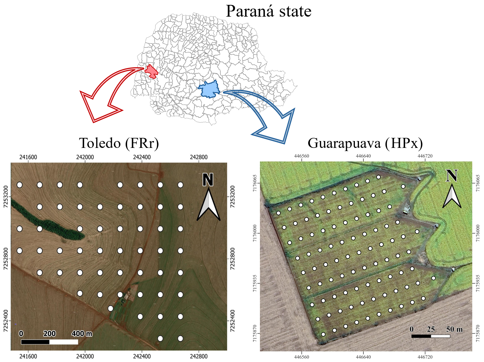
Agricultural soils from two farms in the Paraná State in Brazil were considered individually. In Guarapuava municipality, Southern Paraná State, we collected soil samples classified as Xanthic Hapludox (HPx), with a clay texture. The area is used for soybean (Glycine max) and corn (Zea mays) plantation in the summer, and wheat (Tricticum aestivum), barley (Hordeum vulgare), and black oats (Avena strigosa) in rotation in the winter season. From the area, 372 samples were obtained from 93 sampling points at four depths: 0-10 cm, 10-20 cm, 20-30 cm, and 30-40 cm.
All the soil samples were submitted to conventional analysis for soil pH, BS (Base Saturation), and CEC (Cation Exchangeable Capacity) quantification, following the reference protocols (da, 2009) at the Soil Science and Plant Nutrition Laboratory from the Agronomy Department at the Universidade Estadual do Centro-Oeste (UNICENTRO).
In Toledo municipality, Western Paraná State, the soil is classified as Rhodic Ferralsol (FRr) derived from basalt. The area is used for soybean and corn plantations in summer, in a crop succession system. A set of 212 samples from 53 sampling points at the same four depths of Guarapuava (0-10 cm, 10-20 cm, 20-30 cm, and 30-40 cm) was collected. The determination of pH, BS, CEC, and SOC (Soil Organic Carbon) were performed by the conventional methods at the Soil Laboratory from Instituto de Desenvolvimento Rural do Paraná, according to the same reference protocols (da, 2009).
All samples were collected manually using augers. Figure 1 shows the collection points in each area.
Instrumentation
Approximately 10 g of soil in packed powder form (pressed manually) were accommodated in XRF cups covered with Mylar film for XRF scanning in the EDXRF spectrometer. The amount of soil sample guarantees an infinite thickness sample for the X-ray energy range considered (Van Grieken & Markowicz, 2001).
The equipment employed was a benchtop Shimadzu EDX 720, with a Si(Li) detector and a Rh target X-ray tube. The measurements were performed in two ranges, one at 15 kV and \(454~\mu\)A to reach the light elements from Na to Sc (called 15kV condition) and another with 50 kV and \(38~\mu\)A to reach elements from Ti to U. All measurements were made in triplicate (then the average values were determined), ambient air and for 100 s in each range. Using the equipment’s internal software, the peak’s net area of the following elements were determined: Al, Si, P, S, K, Ca, Ti, Mn, Fe, Cu, Zn, Sr and Zr.
Statistical and machine learning analysis
Descriptive statistics were applied in the fertility attributes data by conventional methods. Additionally, Pearson correlation coefficients between conventional method values and net peak areas from the elements determined by EDXRF (intensity data) were calculated.
For modeling, the two soil datasets were split into calibration and prediction (or validation) sets using the Kennard-Stone (KS) sampling selection algorithm (Kennard & Stone, 1969). It has been widely used in machine learning modeling as an efficient strategy for representatively splitting original data into reduced sets (dos Santos et al., 2023; Nawar & Mouazen, 2018; Nawar et al., 2022; Ribeiro et al., 2024; Tavares et al., 2025).
The algorithm can be summarized in three steps. In the first step, the Euclidean distance, equation (4), among all samples is computed,
\[ D_{ij}^2 = \sum_{n=1}^N\left(x_{in} - x_{jn}\right)^2\]
where \(n = 1,2,\dots,N\) denotes the variables number (limited by \(N\)) while \(i\) (\(j\)) denotes the \(i\)-th (\(j\)-th) sample (\(i\neq j\)). In the second step, the farthest samples are used to define a selection boundary. In the third step, the second farthest samples (limited by the boundary) are included in the subset. Steps two and three are iteratively repeated until the desired number of samples in the subset is reached. This process favors an adequate coverage of the original data variability by the subset, contributing to the robustness and generalization of the models.
The HPx samples were split in approximately \(2/3\) for calibration (248 samples) while the remaining samples were used for prediction (124 samples). Similarly, approximately \(1/3\) of the FRr samples were divided for prediction (72 samples) and the rest (140 samples) were used to calibrate the models. The splitting processes were performed in the matrix encompassing the fertility attributes and independently in the two datasets.
The MLR was performed considering the intensity data. Several strategies were tested in order to optimize the variables which most contribute for each attribute of interest. They were: net areas of all detected elements (Al, Si, P, S, K, Ca, Ti, Mn, Fe, Cu, Zn, Sr, Zr) plus the Compton and Rayleigh scatterings; net areas of only detected elements (Al, Si, P, S, K, Ca, Ti, Mn, Fe, Cu, Zn, Sr, Zr); net areas of the detected elements (Al, Si, P, S, K, Ca, Ti, Mn, Fe, Cu, Zn, Sr, Zr) normalized by the Compton scattering; and net areas of the elements considered significant (95 % confidence level) with a t-test individually applied in soil each attribute model. The modeling with significant variables achieved the highest performance for all soil properties simultaneously, thus, it was used. Full details can be found in the Appendix.
PLS, SVM and RF modeling was performed with the spectra obtained at 15 kV condition. For eliminating noise, the range used was 0.5-10.0 keV, comprising 1260 channels. Poisson scaling followed by mean centering were the preprocessing applied, as recommended by dos Santos (dos Santos et al., 2021). While a 10-fold cross-validation aiming to minimize the RMSE and optimize the number of latent variables was used in PLS, a random grid search was built for defining all hyperparameters of SVM (with linear kernels) and RF. Also minimizing the RMSE with a 10-fold cross-validation, the grid parameter combination was randomly varied 300 times. Full details can be found in the supplementary materials.
The performance of the models was evaluated and indirectly compared by root mean square errors (RMSE), squared correlation coefficients (R\(^2\)) and performance-to-deviation ratio (RPD). Viscarra Rossel et al., 2006 reported that RPD might be used for classifying models as: excellent models (RPD \(>2.5\)), very good models (\(2.5>\) RPD \(>2.0\)), good model \((2.0 >\) RPD \(>1.8\)), fair (\(1.8>\) RPD \(>1.4\)), and very poor model (RPD \(<1.4\)). On the other hand, for directly comparing the model’s performances, the relative improvement in percentage (RI %) coefficients were computed according to equation (5),
\[ \text{RI}\% = \frac{100\times\left(\text{RMSEP}_1 - \text{RMSEP}_2\right)}{\text{RMSEP}_1}\]
in which \(\text{RMSEP}_1\) denotes the RMSE of prediction of the model taken as reference and \(\text{RMSEP}_2\) is the RMSEP of the model to be compared (Ribeiro et al., 2024).
All pre-processing and computational analyses were performed using R Statistical Software (v4.3.3) and Python (v3.11.4). The prospectr R package, version 0.2.7 (Stevens & Ramirez-Lopez, 2024), was used to split the samples with Kennard-Stone algorithm. The stats R package, version 4.3.3 (R, 2024), was used to perform MLR. The datools R package, version 0.14.1, (Kucheryavskiy, 2020) was used to perform PLS as well as the scikit-learn Python library, version 1.4.2, (Pedregosa et al., 2011), was used to perform SVM and RF.
Results
Conventional method results
Box plots of Figure 2 were built to assess the distribution of conventional results and gain perspective on modeling performances. Full descriptive statistics were presented in the supplementary materials.
| (a) | (b) | (c) | (d) |
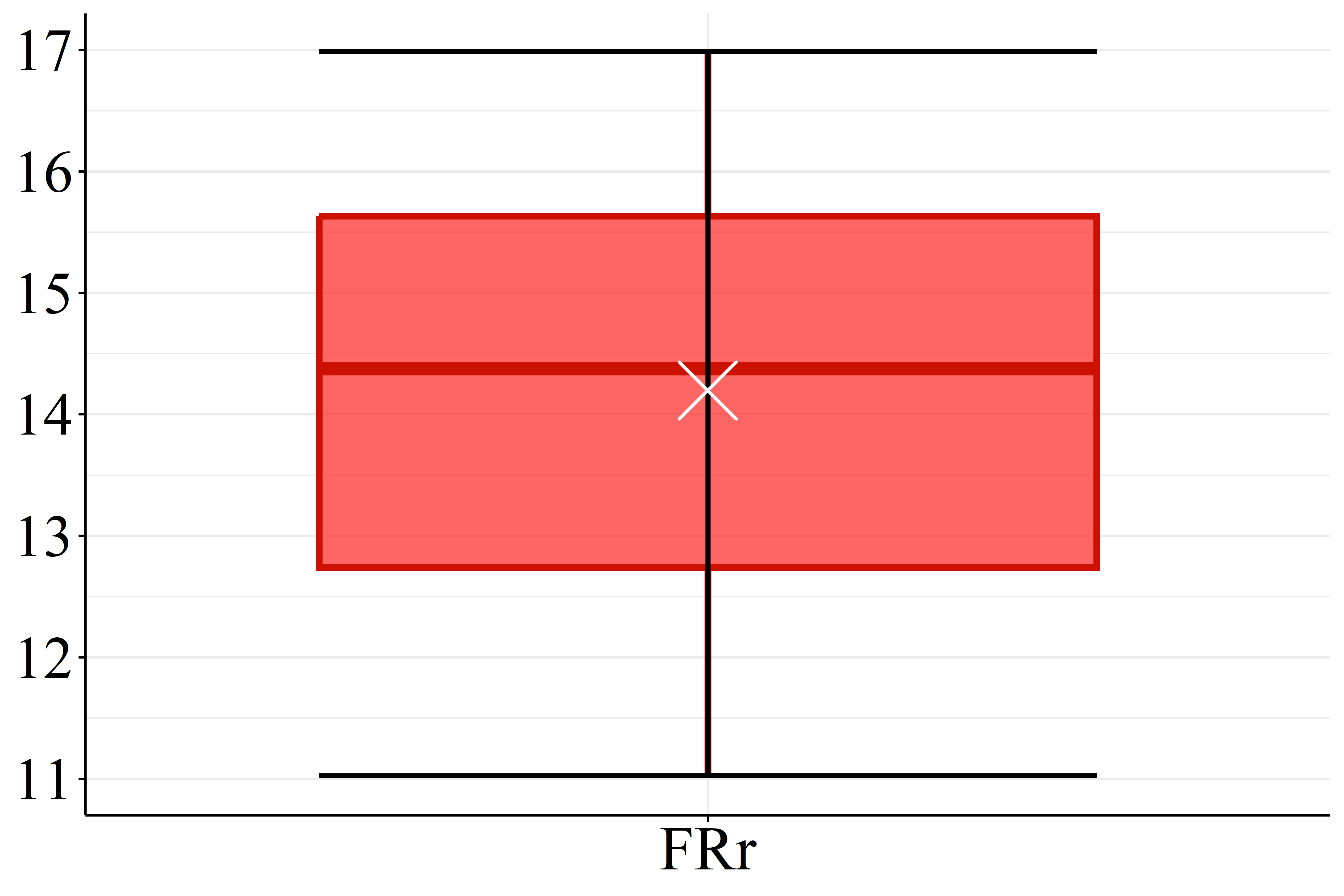 | 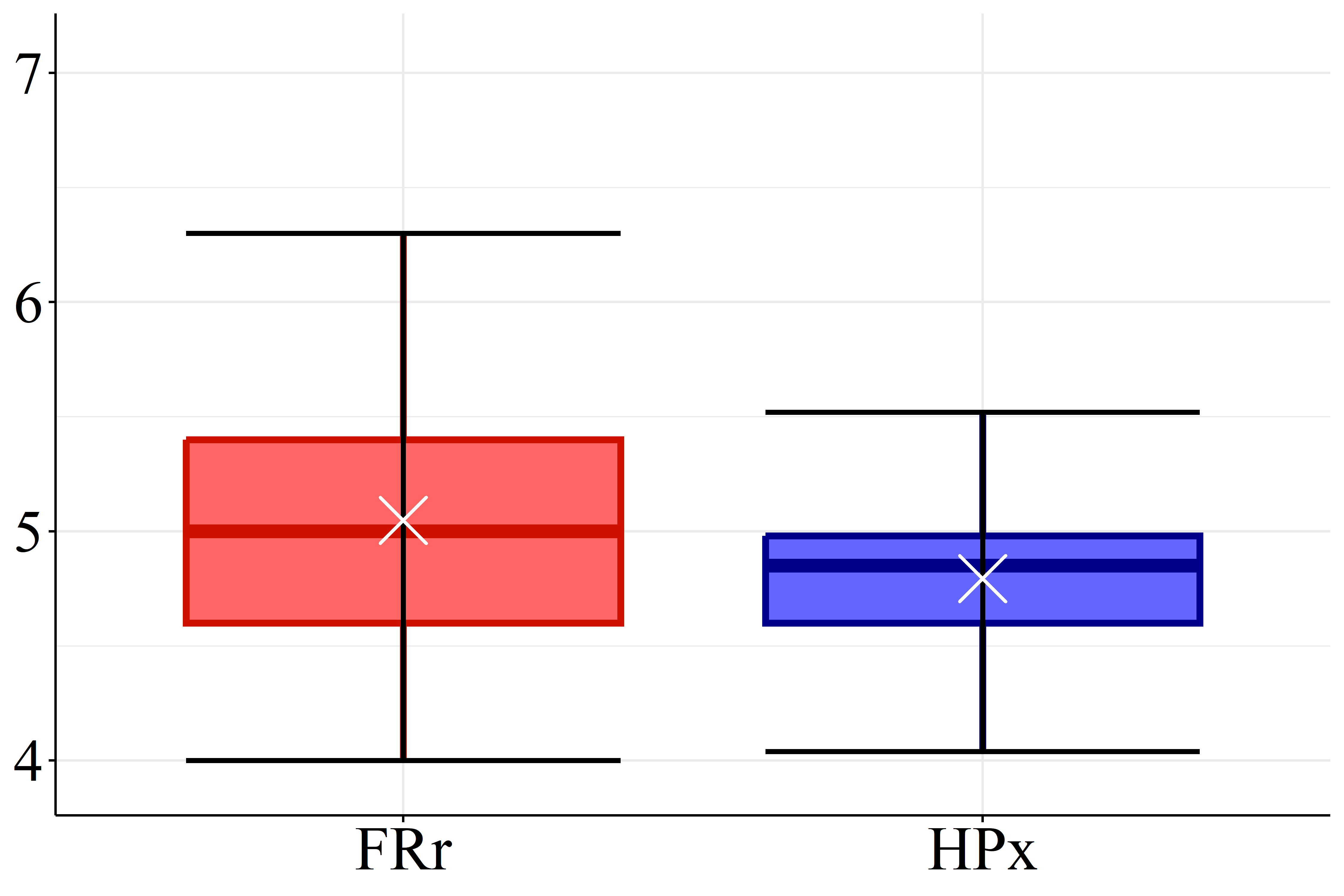 | 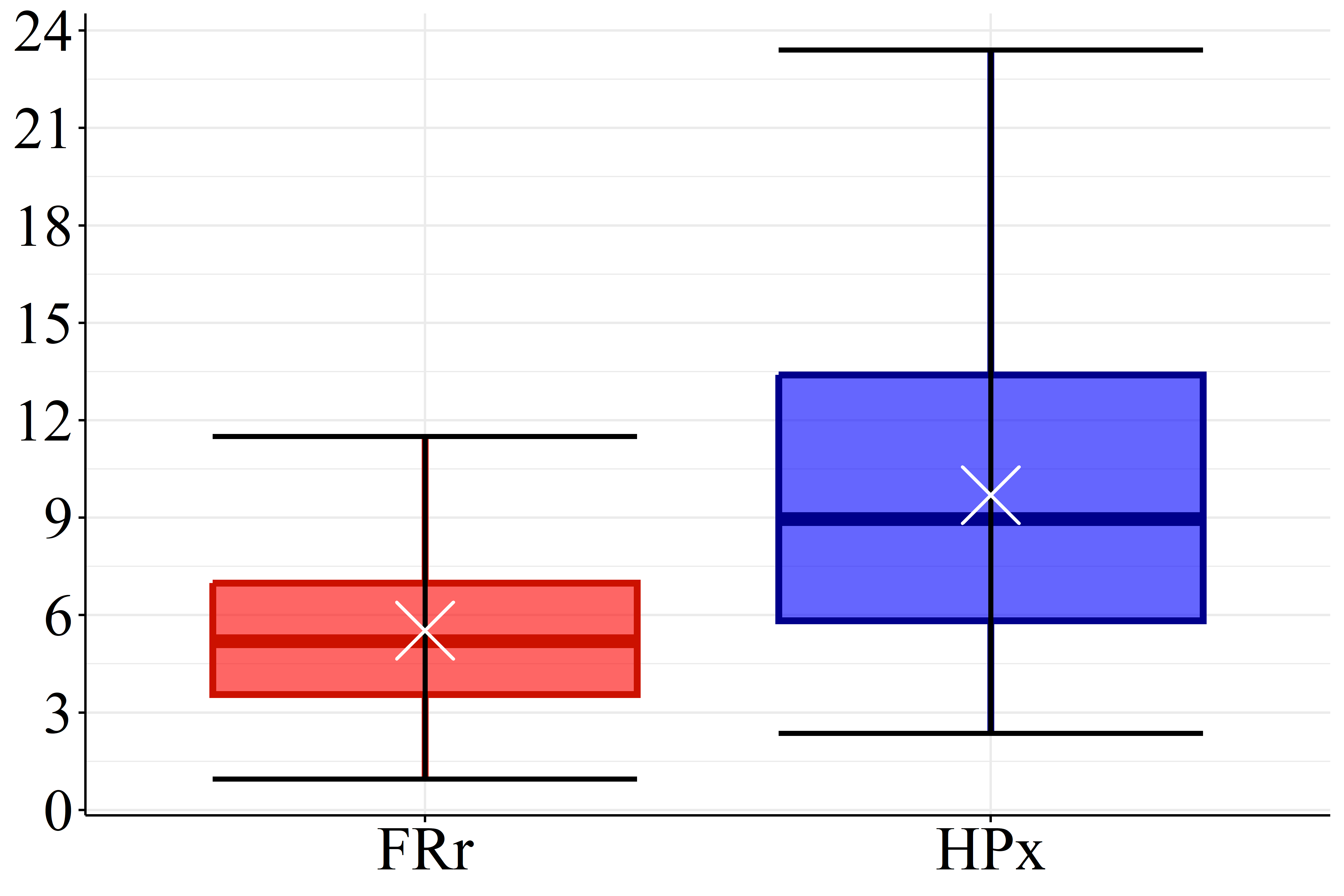 | 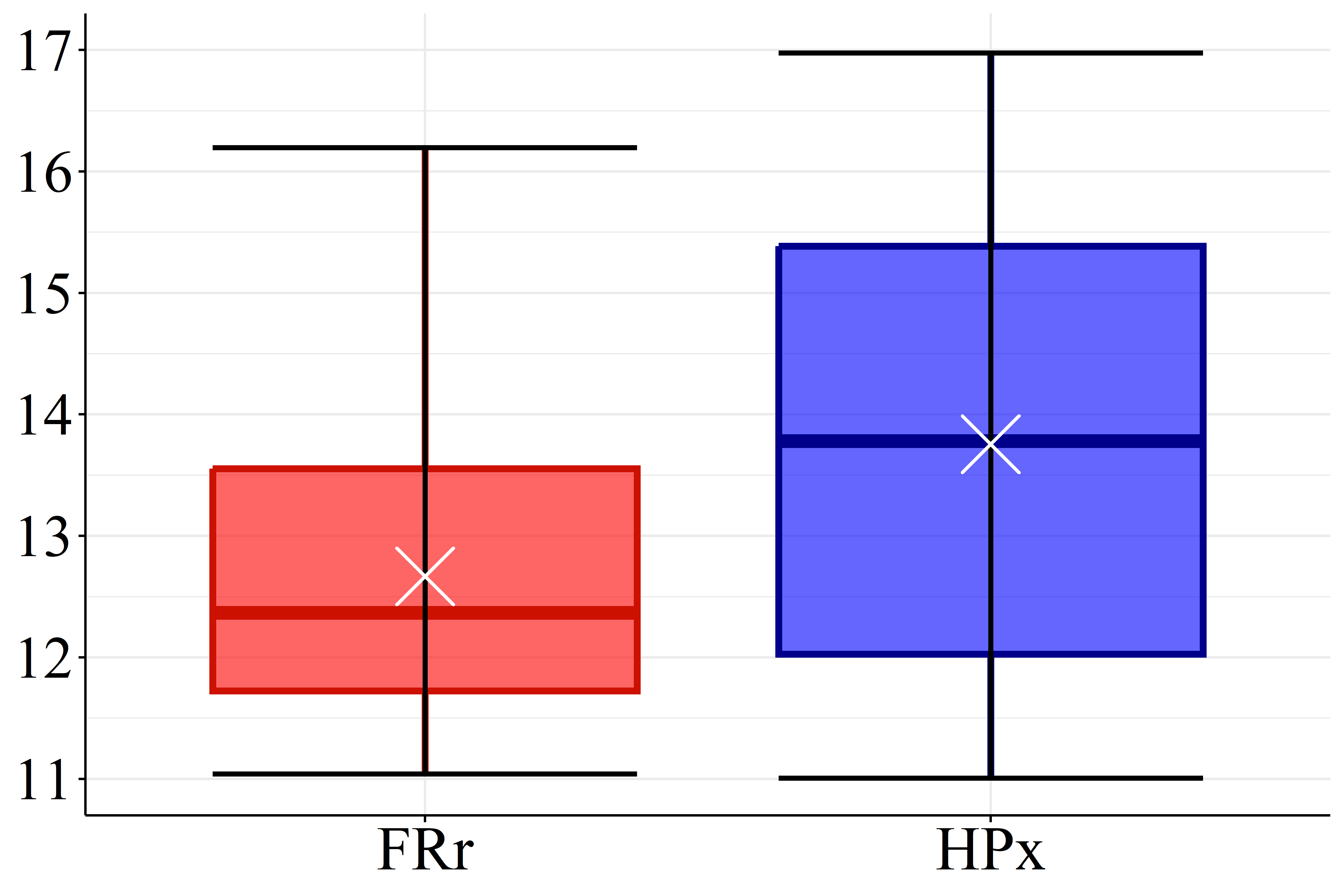 |
According Figure 2(a) the SOC levels of FRr samples (17.1 g.dm\(^{-3}\)) are considered high compared to the reference for Paraná soils (Pavinato et al., 2017). Furthermore, the datasets presented mean pH values lower than 5.1, Figure 2(b), which is considered low (Pavinato et al., 2017), revealing the acidic character of these soils. Figure 2(c) and 2(d) show that both CEC and BS mean values for HPx data (16.5 and 9.7 cmol\(_c.\)dm\(^{-3}\), respectively) are greater than FRr ones (10.7 and 5.5 cmol\(_c.\)dm\(^{-3}\), respectively). On the other hand, most of CEC HPx results are considered high compared to the reference for Paraná soils while CEC FRr values are medium (Pavinato et al., 2017). Since BS indicates the amount of basic nutrients available in the soil and CEC measures its capacity to retain and supply nutrients to plants, these results indicate that HPx soils have greater nutrient availability for plants than FRr soils, and are, therefore, more fertile (Ronquim, 2010).
EDXRF results
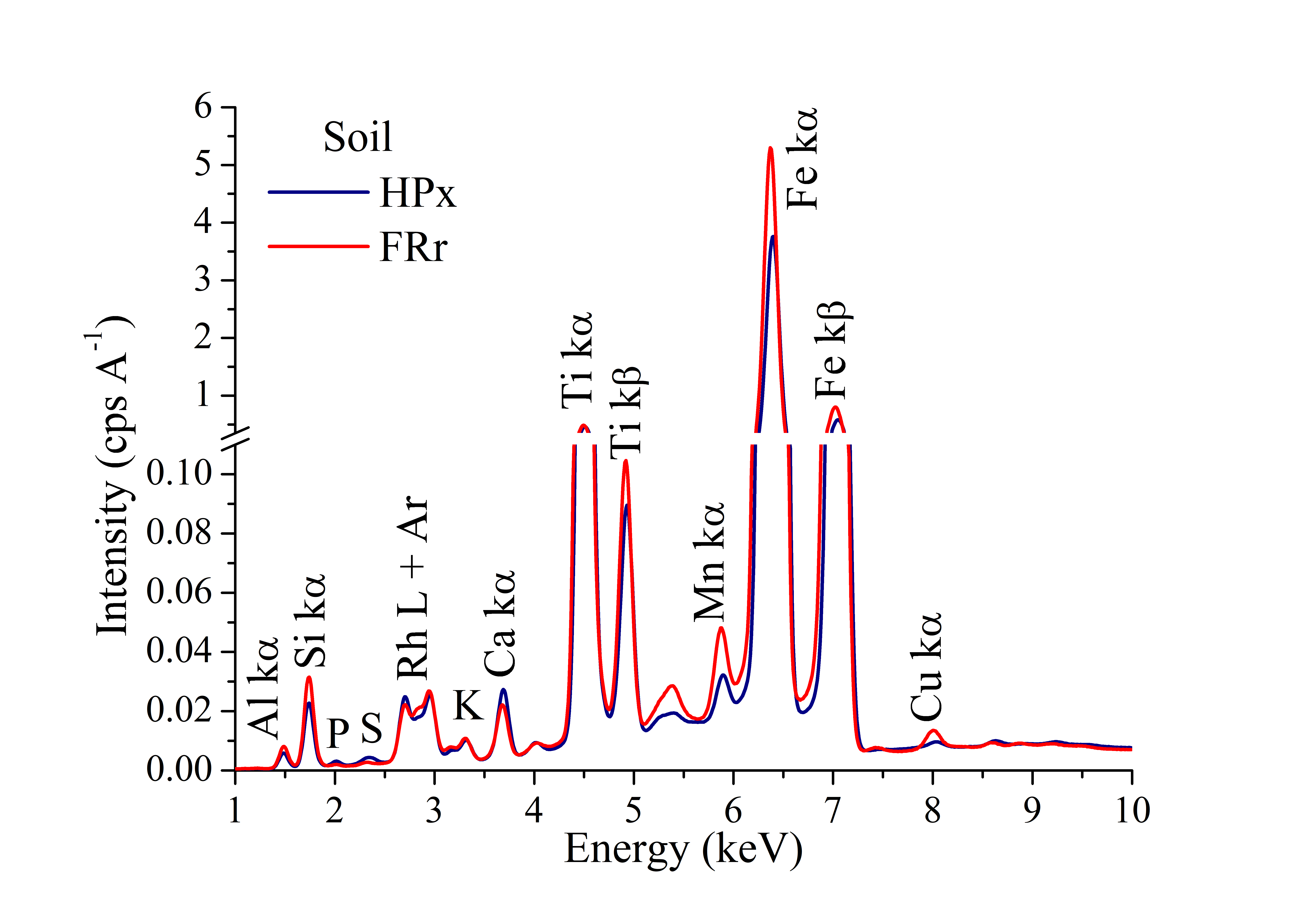
The mean EDXRF spectra at 15 kV condition are shown in Figure 3. The detected elements were: Al, Si, P, S, K, Ca, Ti, Mn, Fe, and Cu, in which Fe, Ti, and Si were found in higher levels. This is attributed to soil profile, rich in iron and aluminum oxides, and high mineral fraction, since the basis of the structure of most clay minerals is Si (Mauad et al., 2003; Prezotti & Guarçoni, 2013). In lower orders, the contents of K, Ca, and Mn were also quantified. In the analyzed soil, these may be related to several sources, such as the clay fraction mineralogy, texture, organic matter, and mainly fertilizers.
Correlograms
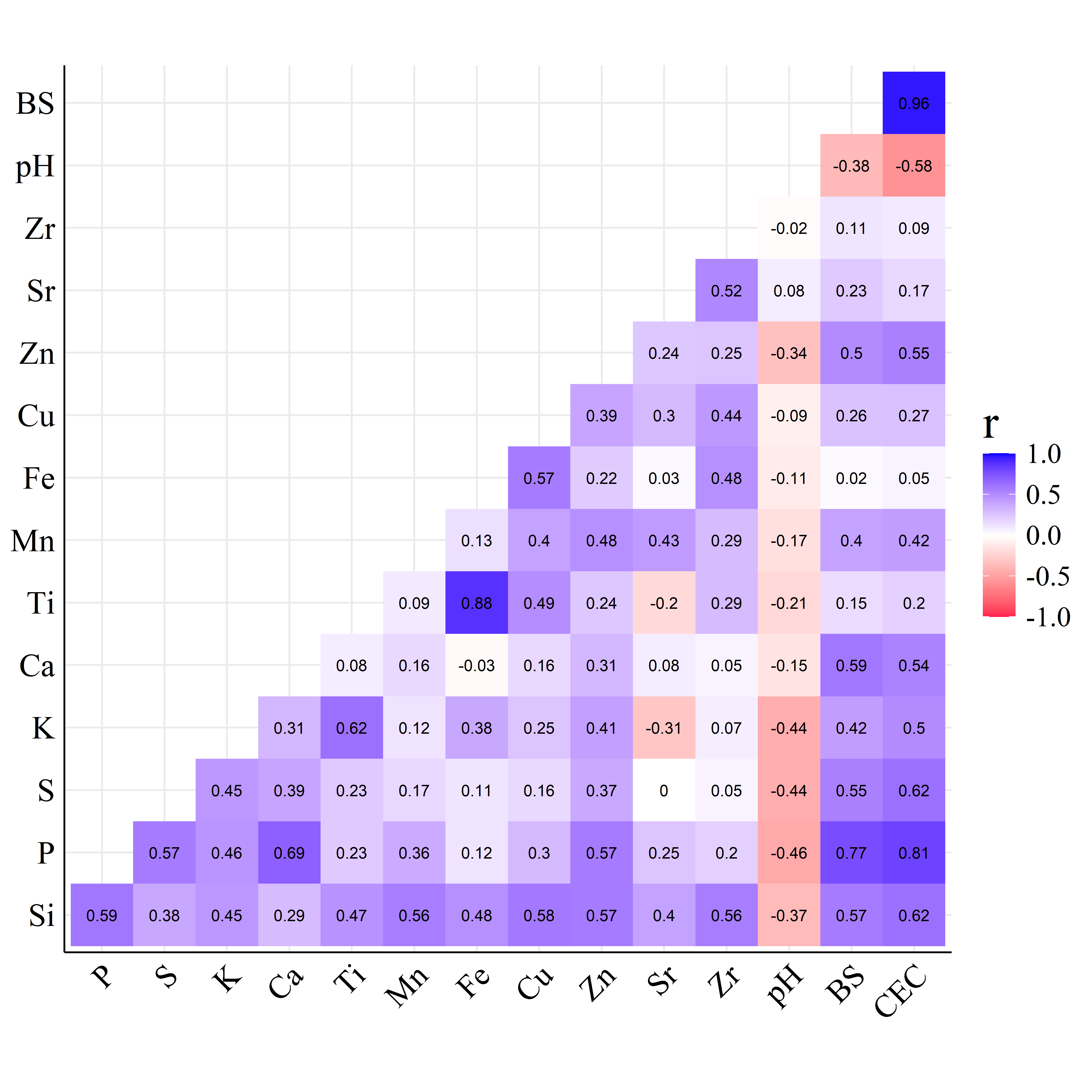
Figure 4 shows the Pearson correlation coefficients between fertility attributes (reference method results) and net area elemental intensities (EDXRF results).
| (a) | (b) |
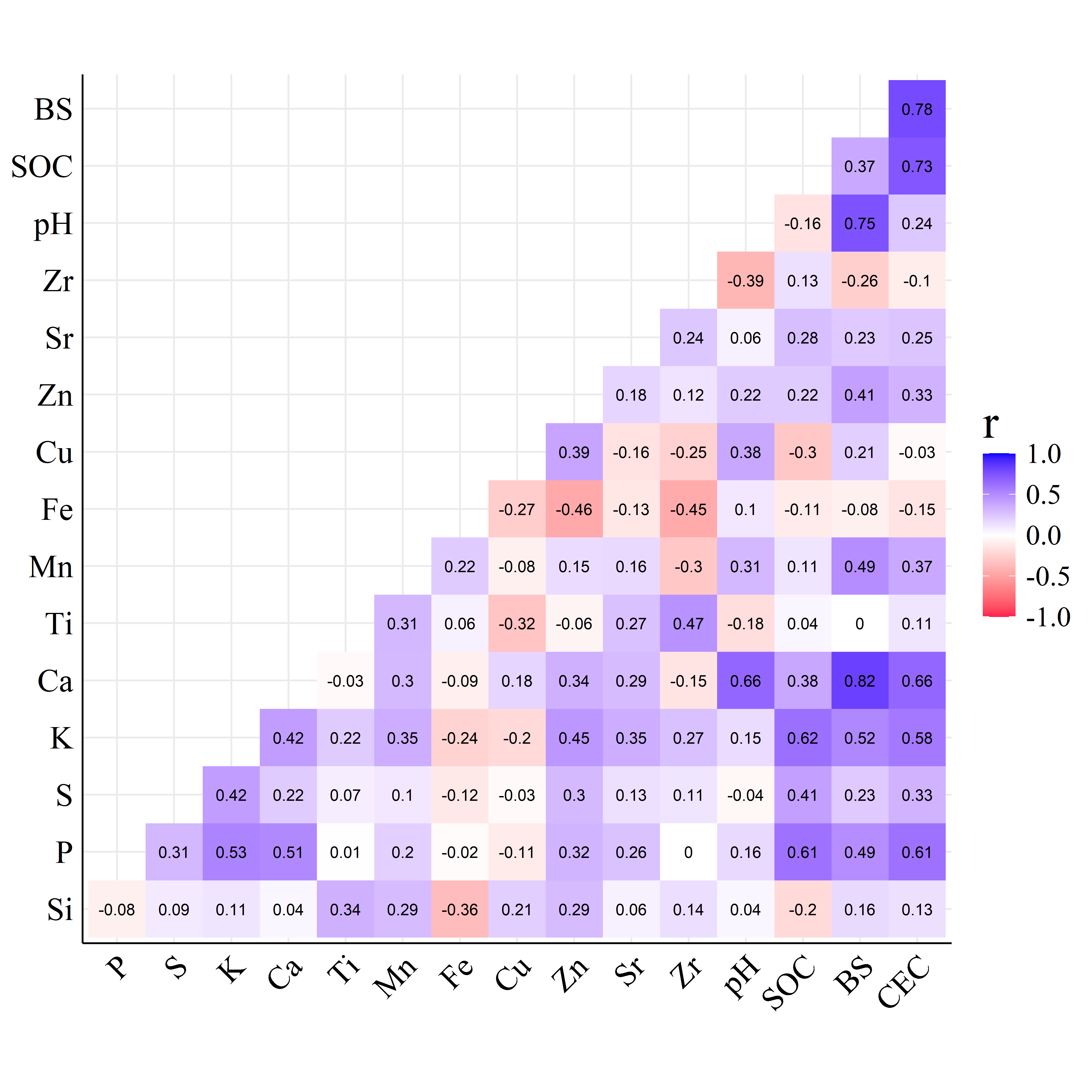 |  |
In the FRr correlogram of Figure 4(a), BS presented the highest correlation coefficient with total Ca (\(r=0.82\)) and total K (\(0.52\)), the exact elements used in BS calculation, as well as P (\(r=0.49\)), Mn (\(0.49\)) and Zn (\(0.41\)) had median correlation values. For CEC the P (\(r=0.61\)), K (\(0.58\)) and Ca (\(0.66\)) had the highest correlation coefficients. Compared with other soil attributes, pH had the lowest correlation with all EDXRF variables simultaneously, presenting only high correlation with Ca (\(r=0.66\)). On the other hand, P and K (\(r>0.6\)) were the main element correlated with SOC.
Similarly, in the HPx correlogram of Figure 4(b), BS had high correlation with Si, P, S, Ca and Zn (\(r>0.50\)) indicating that cations from these elements may be available resulting in high BS values (Sociedade, 2004). In HPx soil the pH has negative correlation with P, S, and K while CEC presents positive correlations with Si, P, S, K and Ca.
Furthermore, accentuated differences are noted between the correlation plots of Figure 4. The mutual correlations among all variables of the HPx samples are more intense compared to the FRr, which may be attributed to the particular characteristics of each soil type.
Modelling performance
Table 1 shows the RMSE, and R\(^2\) results across the different machine learning regression methods as well as the soil dataset. Through these results it was possible to directly compare the performance of the models.
0.18cm
| Xanthic Hapludox soil (HPx) | Rhodic Ferralsol soil (FRr) | ||||||||
|---|---|---|---|---|---|---|---|---|---|
| Attribute | Model | RMSEC | RMSEP | R\(^2\) cal | R\(^2\) pred | RMSEC | RMSEP | R\(^2\) cal | R\(^2\) pred |
| pH | MLR | 0.26 | 0.20 | 0.37 | 0.24 | 0.33 | 0.37 | 0.68 | 042 |
| PLS | 0.15 | 0.19 | 0.77 | 0.33 | 0.24 | 0.33 | 0.86 | 0.40 | |
| SVM | 0.24 | 0.21 | 0.45 | 0.13 | 0.39 | 0.31 | 0.65 | 0.45 | |
| RF | 0.09 | 0.34 | 0.91 | 0.12 | 0.48 | 0.44 | 0.47 | 0.01 | |
| SOC | MLR | - | - | - | - | 3.72 | 3.72 | 0.66 | 0.34 |
| PLS | - | - | - | - | 2.90 | 3.65 | 0.79 | 0.32 | |
| SVM | - | - | - | - | 0.96 | 3.69 | 0.97 | 0.30 | |
| RF | - | - | - | - | 1.87 | 4.10 | 0.91 | 0.13 | |
| BS | MLR | 2.67 | 2.58 | 0.68 | 0.59 | 1.33 | 0.99 | 0.79 | 0.73 |
| PLS | 1.78 | 2.00 | 0.85 | 0.75 | 0.80 | 0.87 | 0.92 | 0.78 | |
| SVM | 1.17 | 2.50 | 0.93 | 0.60 | 1.26 | 1.35 | 0.80 | 0.48 | |
| RF | 1.17 | 3.94 | 0.93 | 0.03 | 0.70 | 1.83 | 0.93 | 0.05 | |
| CEC | MLR | 2.69 | 2.32 | 0.77 | 0.72 | 1.36 | 1.17 | 0.60 | 0.45 |
| PLS | 1.45 | 1.87 | 0.93 | 0.82 | 1.03 | 1.44 | 0.76 | 0.45 | |
| SVM | 1.42 | 2.51 | 0.93 | 0.67 | 1.12 | 1.40 | 0.72 | 0.12 | |
| RF | 1.29 | 4.41 | 0.94 | 0.01 | 0.98 | 1.51 | 0.79 | 0.01 | |
Units: SOC (g.dm\(^{-3}\)), BS and CEC (cmol\(_c\).dm\(^{-3}\)); RMSEC (RMSE of calibration), RMSEP (RMSE of prediction), R\(^2\) cal (R\(^2\) of calibration), and R\(^2\) pred (R\(^2\) of prediction)
It is noted in Table 1 that pH and SOC models presented lower performance results compared with BS and CEC, with RMSEP (R\(^2\) of prediction) ranging from 0.19-0.44 cmol\(_c.\)dm\(^{-3}\) (0.01-0.45) and ranging from 3.65-4.10 g.dm\(^{-3}\) (0.13-0.34), respectively. Conversely, CEC and BS models presented successful results (R² of prediction \(> 0.75\)) (Fontenelli et al., 2021), especially with PLS, and MLR algorithms. On the one hand, BS and CEC are directly related to the bioavailable Ca\(^{2+}\) and K\(^+\) contents, which in turn are related to the characteristic X-ray lines of Ca and K in the EXRF spectrum (Figure 4. On the other hand, there are no EDXRF variables directly related to pH and SOC, and thus, machine learning algorithms seek correlations with other variables such as S and P (Figure 4 to quantify these soil attributes, and this may be related to the low performance in their prediction. In pH case, this low performance might also be associated with the soil samples presenting low pH variations throughout entire datasets (Figure 2 showed that both soil datasets presented a low interquartile range, being \(0.38\) for HPx and \(0.8\) for FRr samples), which is problematic for ML modeling as it may limit the model’s ability to learn broader patterns, leading to overfitting and poor generalizations. Other studies have also reported low pH modeling performances with EDXRF data from soil samples (dos Santos et al., 2020; Ribeiro et al., 2024).
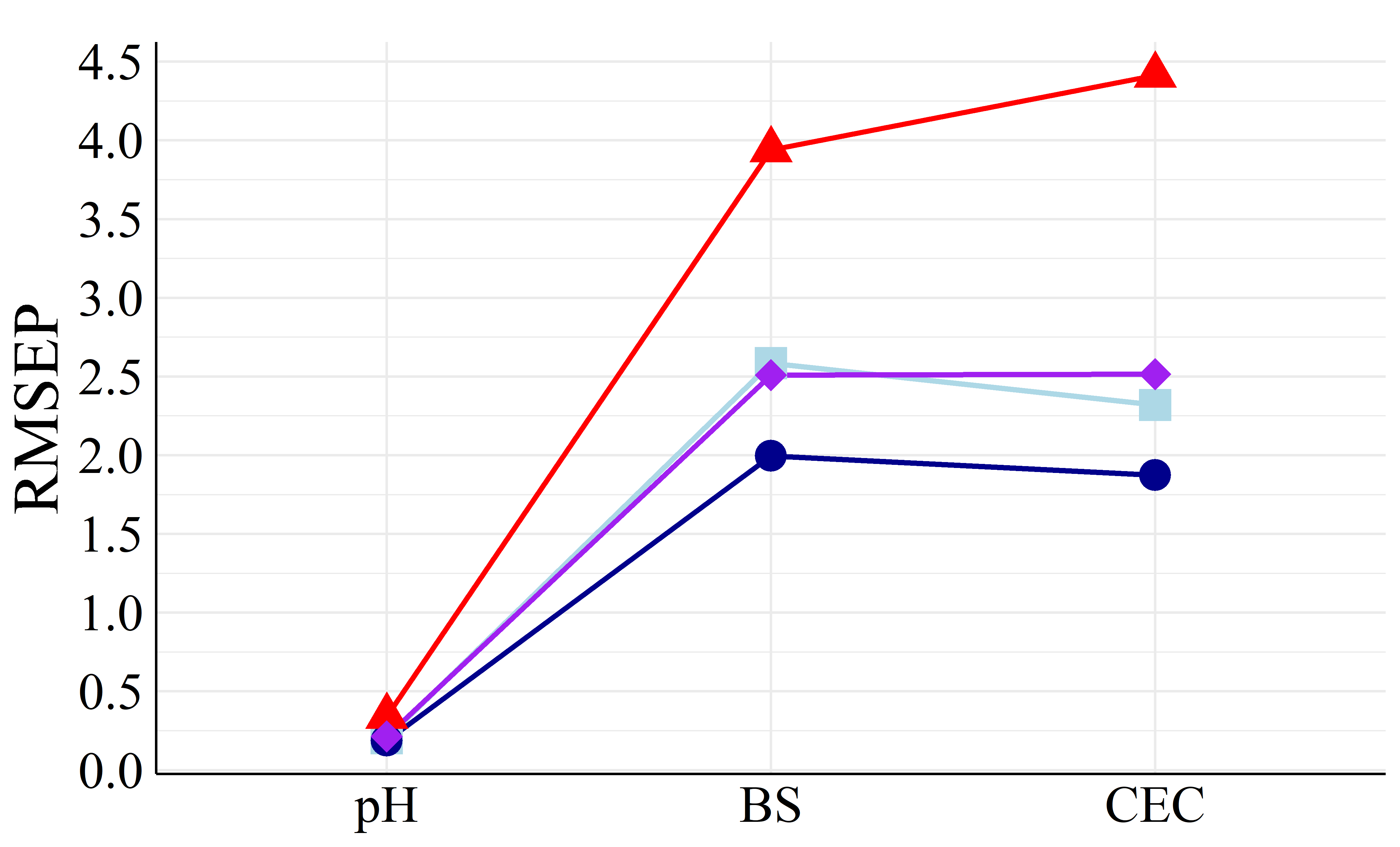
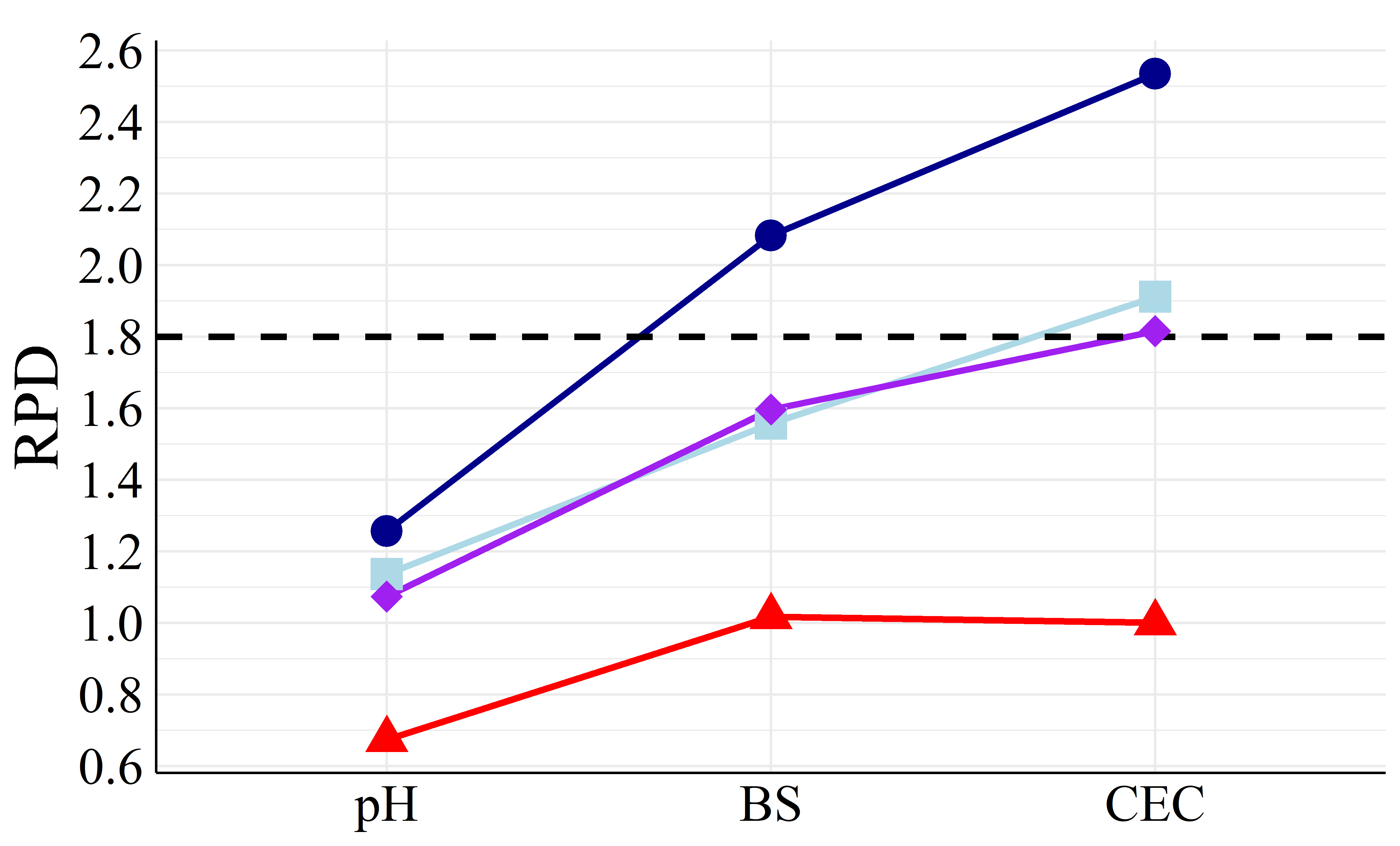
To better visualize the differences in accuracy, Figure 5 presents the different RMSEP and RPD values among all machine learning models.
| (a) | (b) |
 |  |
| (c) | (d) |
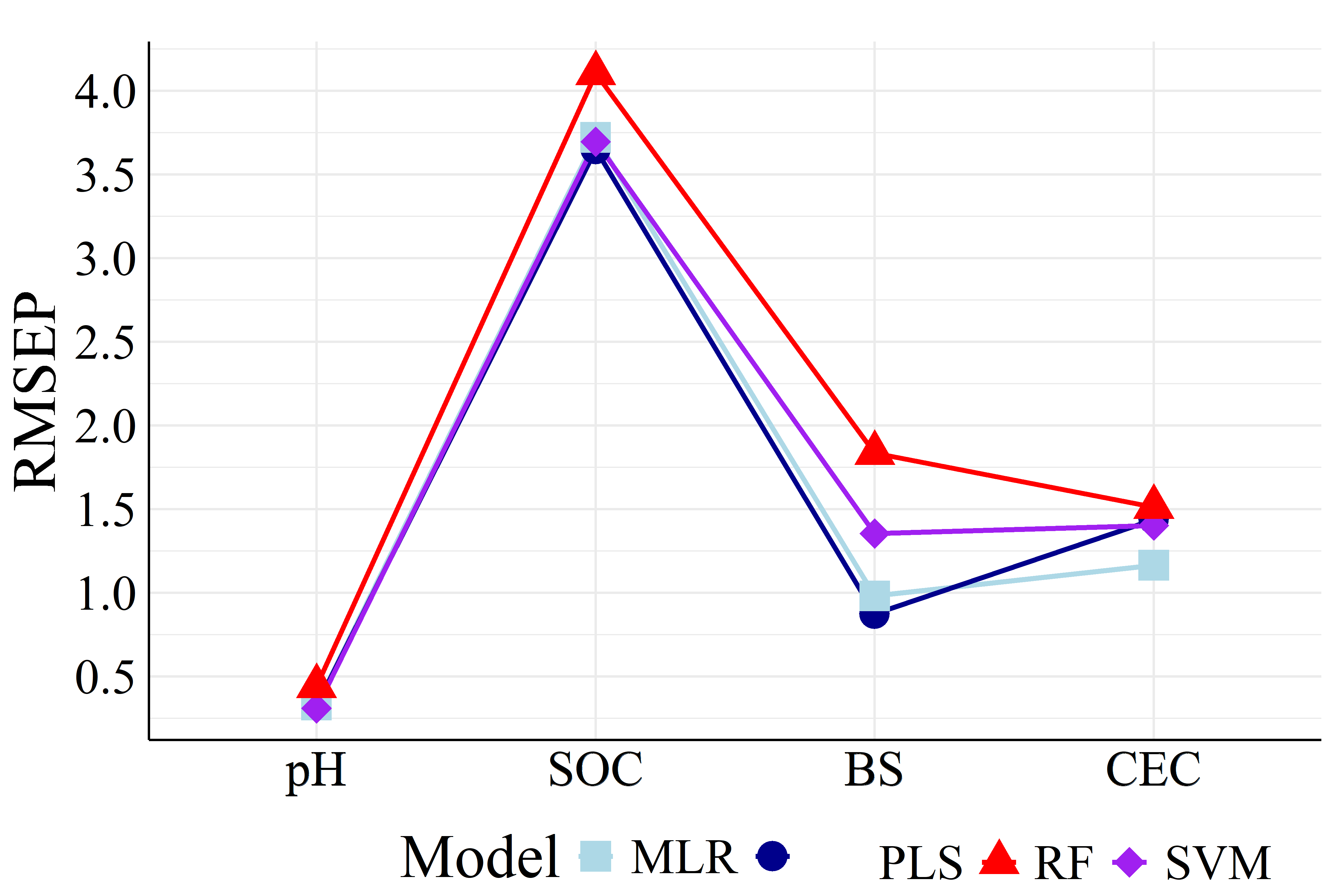 | 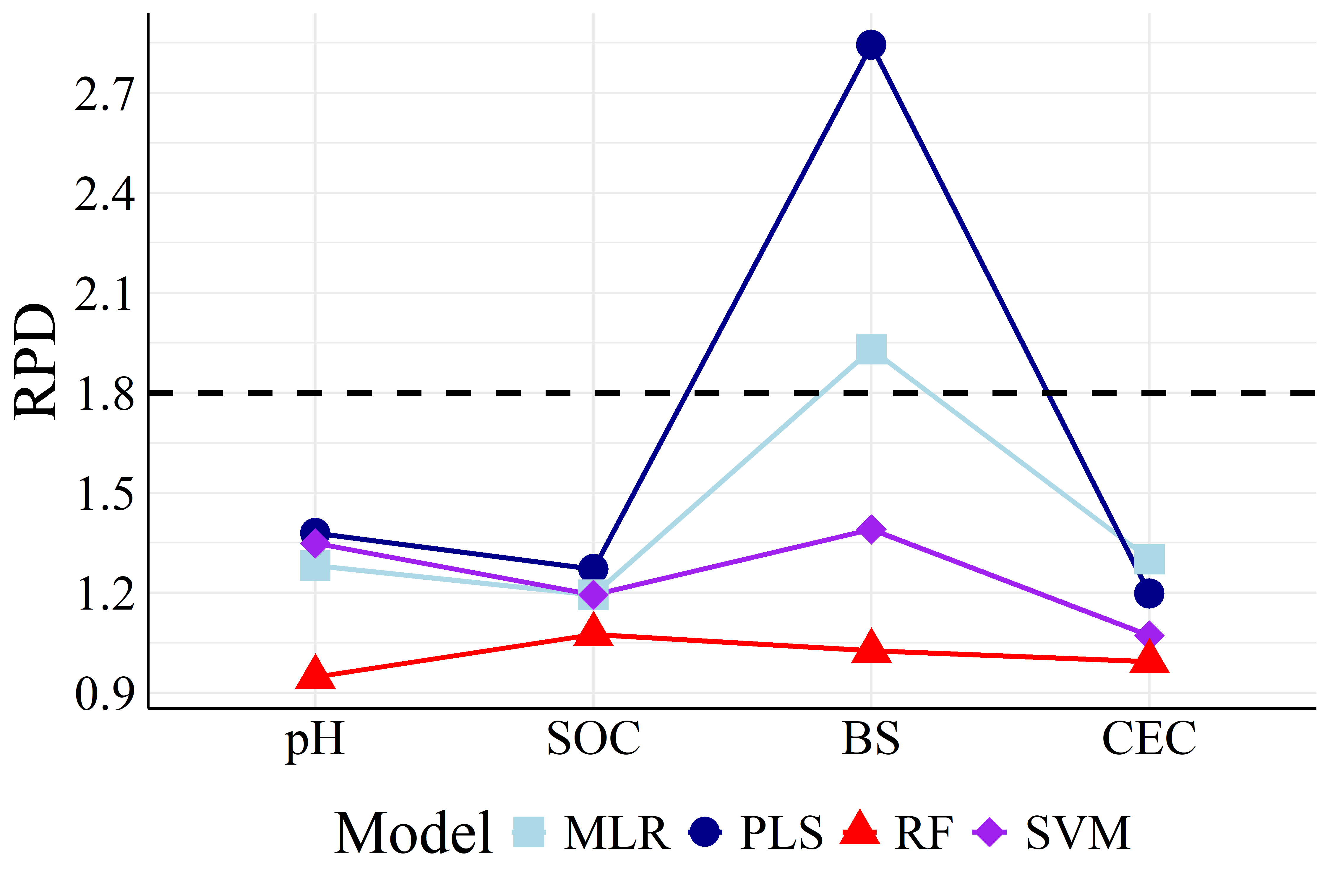 |
It is showed in Figure 5 that PLS achieved both the highest RPD and lowest RMSEP values in most cases compared to the other models, being the best calibration strategy. Apart from PLS models, MLR and SVM performed similarly (except BS models with FRr samples) as well as RF had the worst prediction results. For HPx samples, Figures 5(a) and 5(b), BS and CEC PLS models presented RPD of \(2.08\) and \(2.53\), respectively, considered as very good (RPD \(>2.0\)), i.e., suitables for quantitative analysis (Viscarra Rossel et al., 2006). Among FRr samples, Figures 5(c) and 5(d), only BS models reached high RPD, with values of \(2.84\) (PLS) and \(1.93\) (MLR), considered as excellent and good, respectively (Viscarra Rossel et al., 2006). The remaining models presented RPD lower than \(1.8\) for both HPx and FRr samples.
On the other hand, RI% values, Table 2, quantitatively established PLS as the best modeling strategy, as it did not show improvement in most comparisons with the other ML algorithms. The only exceptions were pH and CEC SVM models and CEC MLR model, which were built with FRr samples. Therefore, even though these models showed improvements compared to PLS (RI% of \(6.06\), \(2.78\), and 18.75 %, respectively), they remained very poor (RPD \(<1.4\)).
| RI% | pH | SOC | BS | CEC |
|---|---|---|---|---|
| Comparison | Xanthic Hapludox soil (HPx) | |||
| PLS x SVM | -10.53 | - | -25.00 | -34.22 |
| PLS x RF | -78.95 | - | -97.00 | -135.83 |
| PLS x MLR | -5.26 | - | -29.00 | -24.06 |
| Rhodic Ferralsol soil (FRr) | ||||
| PLS x SVM | 6.06 | -1.10 | -55.17 | 2.78 |
| PLS x RF | -33.33 | -12.33 | -110.34 | -4.86 |
| PLS x MLR | -12.12 | -1.92 | -13.79 | 18.75 |
This hierarchy of accuracy (PLS\(>\)MLR\(>\)SVM\(>\)RF) might be related to the ability of algorithms to fit the EDXRF while maintaining a balance between underfitting and overfitting. Several studies have reported good performances of PLS for predicting fertility attributes (de Santana et al., 2021; dos Santos et al., 2020; Eitelwein et al., 2022; Ribeiro et al., 2024).
Conversely, the complexity of SVM and RF is significantly higher than that of PLS, presenting several hyperparameters to tune. Thus, their margin for adequate adjustment of calibration conditions that are generalizable for reliable validation is smaller. For instance, although a randomly grid search was used to seek the best parameters, the RF models presented a significant tendency to overfitting in most cases, see Table 1.
Furthermore, spectral data encompass the complex matrix existing in a soil sample (e.g., small differences in organic and mineral materials) better than intensity data (Ribeiro et al., 2024), which may explain the superiority of PLS compared to MLR models.
In summary, this study demonstrated the effectiveness of combining PLS with EDXRF to assess key soil fertility attributes. This alternative method allows for reducing the number of samples submitted to conventional soil analyses, only for model calibration. Once calibrated, future analyses in the same area can be conducted using EDXRF spectra, prepared similarly to the initial calibration step.
In our study, \(2/3\) of the sample sets were chosen to calibrate the models, which would reduce conventional analyses by around \(1/3\). However, further studies addressing the minimum number of samples to calibrate ML models are needed. Even smaller sample sets may be feasible to generate accurate predictions.
This approach may speed up the analysis process and provide results at timely intervals for rational soil management decisions. Furthermore, it enables the analysis of a larger number of samples at a lower cost, increasing efficiency and scalability in agricultural practices. This may directly impact the improvement of soil health monitoring methods.
Conclusions
The study explored four of the most used machine learning tools to the indirect prediction of pH, SOC, BS and CEC from EDXRF data. The different regression models performance revealed that the CEC and BS models, especially those built with the PLS algorithm, presented the best performance, with RPDs higher than \(2.0\), classifying them as suitable for quantitative analyses. In contrast, the pH and SOC models showed lower performances.
Among the algorithms evaluated, PLS stood out as the best calibration strategy, outperforming MLR, SVM and RF in terms of R\(^2\), RMSEP and RPD in most cases. The PLS also proved to be superior regarding the two soil classes evaluated. This superiority might be attributed to its ability to balance the adjustment between underfitting and overfitting, especially when dealing with the complexity of EDXRF spectral data.
This study highlights the potential of combining PLS with EDXRF to reduce the need for conventional soil analyses, being able to speed up the analysis, deliver timely results for soil management, and increase the number of samples analyzed at a lower cost.
Appendix
This Appendix provides detailed supplementary information supporting the modeling analyses and descriptive statistics discussed in the main text. Tables 3 through 9 offer complete data on the modeling methods, parameter ranges, and fertility attribute statistics, enhancing the modeling performance insights shown in Figure 2.
| Samples | Atributte | Significant explained | Total sum of |
| variables (intensity data) | explained variables | ||
| FRr | pH | P, S, Ca, Ti, Fe, Cu | 6 |
| FRr | SOC | Si, P, S, K, Fe, Cu | 6 |
| FRr | BS | Al, Si, K, Ca, Zr | 5 |
| FRr | CEC | Si, P, K, Ca, Ti, Zn, Zr | 7 |
| HPx | pH | P, S, Ca, Sr, Rh | 5 |
| HPx | BS | P, S, Si, Fe, Zr | 5 |
| HPx | CEC | Si, P, S, Mn, Fe, Zr | 6 |
| Samples | Atributte | LV | R\(^2\) CV | RMSECV |
|---|---|---|---|---|
| FRr | pH | 6 | 0.69 | 0.36 |
| FRr | SOC | 6 | 0.59 | 4.06 |
| FRr | BS | 5 | 0.64 | 1.26 |
| FRr | CEC | 5 | 0.72 | 9.57 |
| HPx | pH | 6 | 0.22 | 0.19 |
| HPx | BS | 5 | 2.22 | 1.87 |
| HPx | CEC | 6 | 2.28 | 2.00 |
Units: SOC (g.dm\(^{-3}\)), BS and CEC (cmol\(_c\).dm\(^{-3}\));
CV: Cross-Validation
| Parameter | Range | FRx | HPx | ||||||||
| Best | Default | Best | Default | ||||||||
| CEC | BS | SOC | pH | CEC | BS | pH | |||||
| C | [0.1, 10, 60, 70, 80, | 10 | 10 | 120 | 1 | 80 | 100 | 1 | |||
| 90, 100, 110, 120] | |||||||||||
| \(\epsilon\) | [0.7, 0.8, 0.9, 1, 1.1, 1.5, 2] | 1.1 | 0.7 | 0.9 | 0.1 | 0.7 | 1 | 0.1 | |||
| tol | [0.0007, 0.0009, 0.001 | 0.0012 | 0.0007 | 0.001 | 0.003 | 0.0014 | 0.0013 | 0.003 | |||
| 0.0012, 0.0013, 0.0014] | |||||||||||
| R\(^2\) CV | 10-fold | 0.53 | 0.71 | 0.61 | 0.52 | 0.70 | 0.59 | 0.19 | |||
| RMSE CV | 10-fold | 1.47 | 1.55 | 3.97 | 0.46 | 3.06 | 3.04 | 0.29 | |||
Units: SOC (g.dm\(^{-3}\)), BS and CEC (cmol\(_c\).dm\(^{-3}\)); CV: Cross-Validation
| Parameter | Range | FRx | HPx | ||||||||
| Best | Default | Best | Default | ||||||||
| CEC | BS | SOC | pH | CEC | BS | pH | |||||
| n_estimators | [230, 250, 265, 270] | 250 | 265 | 265 | 100 | 230 | 250 | 100 | |||
| max_features | [1, 50, 100, 200] | 50 | 100 | 100 | 1 | 100 | 100 | 1 | |||
| max_depth | (None, 30, 35] | 35 | None | 35 | None | 35 | 35 | None | |||
| min_impurity_decrease | [0.115, 0.125, 0.135] | 0.115 | 0.115 | 0.125 | 0 | 0.115 | 0.115 | 0 | |||
| min_samples_split | [5, 10, 20, 30] | 20 | 5 | 5 | 2 | 5 | 10 | 2 | |||
| R\(^2\) CV | 10-fold | 0.58 | 0.86 | 0.51 | 0.37 | 0.82 | 0.82 | 0.33 | |||
| RMSE CV | 10-fold | 1.39 | 1.08 | 4.44 | 0.53 | 2.39 | 2.01 | 0.26 | |||
Units: SOC (g.dm\(^{-3}\)), BS and CEC (cmol\(_c.\)dm\(^{-3}\)); CV: Cross-Validation
| Parameter | FRr | HPx | FRr | HPx | FRr | HPx | FRr | |||
| pH | BS | CEC | SOC | |||||||
| Mean | 5.0 | 4.8 | 5.5 | 9.7 | 10.7 | 16.5 | 17.1 | |||
| Median | 5.0 | 4.9 | 5.2 | 9.0 | 10.5 | 15.5 | 17.3 | |||
| Standard Deviation | 0.6 | 0.3 | 2.6 | 4.6 | 2.0 | 5.3 | 5.8 | |||
| Kurtosis | 0.9 | 0.0 | 0.0 | -0.9 | -0.3 | -1.0 | -0.2 | |||
| Skewness | 0.8 | -0.5 | 0.7 | 0.4 | 0.3 | 0.4 | 0.2 | |||
| Maximum | 4.0 | 3.9 | 1.0 | 2.4 | 6.6 | 6.0 | 3.8 | |||
| Minimum | 7.1 | 5.6 | 14.2 | 23.4 | 16.2 | 29.5 | 34.0 | |||
| Element | Mean\(\pm\)SD | CV | Max | Min | Kurt | Skew |
|---|---|---|---|---|---|---|
| Al | 0.055\(\pm\)0.005 | 9% | 0.068 | 0.042 | -0.223 | -0.432 |
| Si | 0.24\(\pm\)0.03 | 10% | 0.32 | 0.18 | -0.32 | -0.19 |
| P | 0.015\(\pm\)0.005 | 33% | 0.038 | 0.007 | 1.677 | 1.078 |
| S | 0.027\(\pm\)0.006 | 22% | 0.062 | 0.012 | 8.641 | 1.769 |
| K | 0.082\(\pm\)0.014 | 17% | 0.129 | 0.051 | 0.303 | 0.596 |
| Ca | 0.3\(\pm\)0.2 | 88% | 3.1 | 0.1 | 84.9 | 8.0 |
| Ti | 22.8\(\pm\)1.8 | 8% | 26.9 | 18.1 | -0.3 | -0.3 |
| Mn | 0.735\(\pm\)0.150 | 20% | 1.904 | 0.382 | 10.428 | 1.707 |
| Fe | 385\(\pm\)22 | 6% | 428 | 320 | -0.2 | -1 |
| Cu | 0.51\(\pm\)0.05 | 9% | 0.65 | 0.38 | -0.22 | -0.07 |
| Zn | 0.46\(\pm\)0.08 | 17% | 1.12 | 0.31 | 15.70 | 2.60 |
| Sr | 0.9\(\pm\)0.2 | 19% | 1.3 | 0.5 | -0.6 | -0.1 |
| Zr | 16.0\(\pm\)0.6 | 4% | 17.0 | 13.1 | 0.7 | -0.5 |
Med = median, SD = Standard deviation, CV = coefficient of variation,
Max = Maximum, Min = Minimum, Kurt = Kurtosis, Skew = Skewness.
| Element | Mean\(\pm\)SD | CV | Max | Min | Kurt | Skew |
|---|---|---|---|---|---|---|
| Al | 0.081\(\pm\)0.008 | 10% | 0.058 | 0.098 | -0.041 | -0.413 |
| Si | 0.35\(\pm\)0.04 | 11% | 0.24 | 0.46 | 0.33 | 0.05 |
| P | 0.007\(\pm\)0.003 | 48% | 0.001 | 0.018 | -0.211 | 0.569 |
| S | 0.010\(\pm\)0.004 | 36% | 0.000 | 0.021 | 0.422 | 0.105 |
| K | 0.09\(\pm\)0.02 | 25% | 0.04 | 0.16 | 0.39 | 0.81 |
| Ca | 0.20\(\pm\)0.15 | 74% | 0.04 | 1.56 | 33.39 | 4.25 |
| Ti | 24.8\(\pm\)2.7 | 11% | 18.2 | 32.0 | -0.1 | -0.1 |
| Mn | 1.3\(\pm\)0.5 | 40% | 0.6 | 3.3 | 1.0 | 1.2 |
| Fe | 549\(\pm\)22 | 4% | 451 | 611 | 4 | -1 |
| Cu | 1.23\(\pm\)0.14 | 11% | 0.93 | 1.63 | -0.21 | 0.45 |
| Zn | 0.42\(\pm\)0.06 | 14% | 0.25 | 0.64 | 0.91 | 0.31 |
| Sr | 0.17\(\pm\)0.06 | 37% | 0.03 | 0.34 | -0.15 | 0.42 |
| Zr | 5.8\(\pm\)0.4 | 7% | 4.4 | 6.8 | 0.6 | -0.7 |
Med = median, SD = Standard deviation, CV = coefficient of variation, Max = Maximum, Min = Minimum, Kurt = Kurtosis, Skew = Skewness.
Acknowledgments
The authors acknowledge the support CNPq (grant number 306309/2023-8 and 1 50500/2022-0, project number: 404214/2021-5), INCT-FNA (464898/2014-5).
Data availability
Data will be made available on request.
Author contributions
J. V. Ribeiro: Conceptualization, Data curation, Formal analysis, Investigation, Methodology, Programs, Validation, Writing-original draft preparation, Writing-review and editing; F. R. dos Santos: Conceptualization, Methodology, Investigation, Validation, Writing-original draft preparation; J. V. de Oliveira Alves: Data curation, Investigation, Formal analysis, Visualization, Writing-original draft preparation; M. S. Fossaluza: Data curation, Investigation, Formal analysis, Visualization, Writing-original draft preparation; I. M. Nogueira: Data curation, Investigation, Formal analysis, Visualization; J. F. de Oliveira: Methodology, Validation, Writing-review and editing; G. M. C. Barbosa: Methodology, Funding acquisition, Project administration, Resources, Supervision; M. M. L. Müller: Methodology, Investigation, Project administration, Resources, Supervision, Validation, Writing – review and editing; R. A. Borecki: Methodology, Research, Resources; C. A. Pott: Methodology, Research, Project administration, Resources, Resources, Supervision, Validation, Writing – review and editing; F. L. Melquiades: Conceptualization, Data curation, Formal analysis, Methodology, Funding acquisition, Research, Project administration, Resources, Supervision, Validation, Writing – original draft preparation, Writing – review and editing.
Conflicts of interest
The authors declare that they have no known competing financial interests or personal relationships that could have appeared to influence the work reported in this paper.
References
Biau, Gérard & Scornet, Erwan (2016). A random forest guided tour. Springer. 25(2), 197--227. https://doi.org/10.1007/s11749-016-0481-7
da Silva, Francisco César (2009). Manual de análises químicas de solos, plantas e fertilizantes. Brasília, DF: Embrapa Informação Tecnológica; Rio de Janeiro: Embrapa Solos.
Sociedade Brasileira de Ciência do Solo. Núcleo Regional Sul (2004). Manual de adubação e de calagem: para os estados do Rio Grande do Sul e de Santa Catarina. Comissão de Química e Fertilidade do Solo-RS/SC.
de Santana, Felipe B., de Souza, André M. & Poppi, Ronei J. (2018). Visible and near infrared spectroscopy coupled to random forest to quantify some soil quality parameters. 454--462. https://doi.org/10.1016/j.saa.2017.10.052
de Santana, Felipe B., Otani, Sebastião K., de Souza, André M. & Poppi, Ronei J. (2021). Comparison of PLS and SVM models for soil organic matter and particle size using vis-NIR spectral libraries. e00436. https://doi.org/10.1016/j.geodrs.2021.e00436
Demattê, José A. M., Dotto, André C., Bedin, Leonardo G., Sayão, Viviane M. & Souza, Anderson B. (2019). Soil analytical quality control by traditional and spectroscopy techniques: Constructing the future of a hybrid laboratory for low environmental impact. 111--121. https://doi.org/10.1016/j.geoderma.2018.09.010
dos Santos, Felipe R., de Oliveira, Janiel F., Barbosa, Gabriel M. C. & Melquiades, Francisco L. (2021). Comparison between energy dispersive X-ray fluorescence spectral data and elemental data for soil attributes modelling. 106303. https://doi.org/10.1016/j.sab.2021.106303
dos Santos, Felipe R., de Oliveira, Janiel F., Bona, Everson., Barbosa, Gabriel M. C. & Melquiades, Francisco L. (2021). Evaluation of pre-processing and variable selection on energy dispersive X-ray fluorescence spectral data with partial least square regression: A case of study for soil organic carbon prediction. 106016. https://doi.org/10.1016/j.sab.2020.106016
dos Santos, Felipe R., de Oliveira, Janiel F., Bona, Everson., Barbosa, Gabriel M. C. & Melquiades, Francisco L. (2023). Data fusion of XRF and vis-NIR using p-ComDim to predict some fertility attributes in tropical soils derived from basalt. 108813. https://doi.org/10.1016/j.microc.2023.108813
dos Santos, Felipe R., de Oliveira, Janiel F., Bona, Everson., dos Santos, José V. F., Barboza, Gabriel M. C. & Melquiades, Francisco L. (2020). EDXRF spectral data combined with PLSR to determine some soil fertility indicators. 104275. https://doi.org/10.1016/j.microc.2019.104275
Eitelwein, Mariele T., Tavares, Tatiana R., Molin, Júlio P., Trevisan, Renato G., de Sousa, Rubens V. & Demattê, José A. M. (2022). Predictive Performance of Mobile Vis–NIR Spectroscopy for Mapping key Fertility Attributes in Tropical Soils Through Local Models Using PLS and ANN. 3(1), 116--131. https://doi.org/10.3390/automation3010006
Filgueiras, Paulo R., Terra, Luciana A., Castro, Edilene V. R., Oliveira, Luiz M. S. L., Dias, José C. M. & Poppi, Ronei J. (2015). Prediction of the distillation temperatures of crude oils using 1H NMR and support vector regression with estimated confidence intervals. 197--205. https://doi.org/10.1016/j.talanta.2015.04.046
Fontenelli, Júlia V., Adamchuk, Viacheslav I., Ferreira, Marcio M. C., Amaral, Luiz R., Guimarães, Carla C. B., Demattê, José A. M. & Magalhães, Paulo S. G. (2021). Evaluating the synergy of three soil spectrometers for improving the prediction and mapping of soil properties in a high anthropic management area: A case of study from Southeast Brazil. 115347. https://doi.org/10.1016/j.geoderma.2021.115347
Garthwaite, P. H. (1994). An Interpretation of Partial Least Squares. 89(425), 122--127. https://doi.org/10.1080/01621459.1994.10476452
Geladi, P. & Kowalski, B. R. (1986). Partial least-squares regression: a tutorial. 1--17. https://doi.org/10.1016/0003-2670(86)80028-9
Jobson, J. D. (1991). Applied Multivariate Data Analysis. Springer New York. https://doi.org/10.1007/978-1-4612-0955-3
Kennard, R. W. & Stone, L. A. (1969). Computer Aided Design of Experiments. 11(1), 137--148. https://doi.org/10.1080/00401706.1969.10490666
Kucheryavskiy, S. (2020). mdatools — R package for chemometrics. https://doi.org/10.1016/j.chemolab.2020.103937
Mateos-Aparicio, G. (2011). Partial Least Squares (PLS) Methods: Origins, Evolution, and Application to Social Sciences. 40(13), 2305--2317. https://doi.org/10.1080/03610921003778225
Mauad, M., Grassi Filho, H., Crusciol, C. A. C. & Corrêa, J. C. (2003). Teores de silício no solo e na planta de arroz de terras altas com diferentes doses de adubação silicatada e nitrogenada. 27(5), 867--873. https://doi.org/10.1590/S0100-06832003000500011
Melquiades, F. L. & dos Santos, F. R. (2015). Preliminary Results: Energy Dispersive X-Ray Fluorescence and Partial Least Squares Regression for Organic Matter Determination in Soil. 48(4), 286--289. https://doi.org/10.1080/00387010.2013.874532
Morona, F., dos Santos, F. R., Brinatti, A. M. & Melquiades, F. L. (2017). Quick analysis of organic matter in soil by energy-dispersive X-ray fluorescence and multivariate analysis. 13--20. https://doi.org/10.1016/j.apradiso.2017.09.008
Nawar, S. & Mouazen, A. M. (2018). Optimal sample selection for measurement of soil organic carbon using on-line vis-NIR spectroscopy. 469--477. https://doi.org/10.1016/j.compag.2018.06.042
Nawar, S., Richard, F., Kassim, A. M., Tekin, Y. & Mouazen, A. M. (2022). Fusion of Gamma-rays and portable X-ray fluorescence spectral data to measure extractable potassium in soils. 105472. https://doi.org/10.1016/j.still.2022.105472
Oshunsanya, S. O., Oluwasemire, K. O. & Taiwo, O. J. (2017). Use of GIS to Delineate Site-Specific Management Zone for Precision Agriculture. 48(5), 565--575. https://doi.org/10.1080/00103624.2016.1270298
Pavinato, P. S., Pauletti, V., Motta, A. C. V., Moreira, A. & Motta, A. C. V. (2017). Manual de adubação e calagem para o Estado do Paraná. Sociedade Brasileira de Ciência do Solo (SBCS), Núcleo Estadual do Paraná (NEPAR).
Pedregosa, F., Varoquaux, G., Gramfort, A., Michel, V., Thirion, B., Grisel, O., Blondel, M., Prettenhofer, P., Weiss, R., Dubourg, V., Vanderplas, J., Passos, A., Cournapeau, D., Brucher, M., Perrot, M. & Duchesnay, E. (2011). Scikit-learn: Machine Learning in Python. 2825--2830.
Pramod Pawase, P., Nalawade, S. M., Bhanage, G. B., Walunj, A. A., Kadam, P. B., Durgude, A. G. & Patil, M. R. (2023). Variable rate fertilizer application technology for nutrient management: A review. 16(4), 11--19. https://doi.org/10.25165/j.ijabe.20231604.7671
Prezotti, L. C. & Guarçoni, A. M. (2013). Guia de interpretação de análise de solo e foliar. Incaper.
R Core Team (2024). R: A Language and Environment for Statistical Computing.
Ribeiro, J. V., dos Santos, F. R., de Oliveira, J. F., Barbosa, G. M. C. & Melquiades, F. L. (2024). Optimization of pXRF instrumentation conditions and multivariate modeling in soil fertility attributes determination. 106835. https://doi.org/10.1016/j.sab.2023.106835
Ronquim, C. C. (2010). Conceitos de fertilidade do solo e manejo adequado para as regiões tropicais.
Stevens, A. & Ramirez-Lopez, L. (2024). An introduction to the prospectr package (0.2.7). R package Vignette.
Tavares, T. R., Minasny, B., McBratney, A., Molin, J. P., Marques, G. T., Ragagnin, M. M., dos Santos, F. R., de Carvalho, H. W. P. & Lavres, J. (2025). Do XRF local models have temporal stability for predicting plant-available nutrients in different years? A long-term study showing the effect of soil fertility management in a tropical field. 106307. https://doi.org/10.1016/j.still.2024.106307
Tavares, T. R., Molin, J. P., Nunes, L. C., Wei, M. C. F., Krug, F. J., de Carvalho, H. W. P. & Mouazen, A. M. (2021). Multi-Sensor Approach for Tropical Soil Fertility Analysis: Comparison of Individual and Combined Performance of VNIR, XRF, and LIBS Spectroscopies. 11(6), 1028. https://doi.org/10.3390/agronomy11061028
Terra, J., Sanches, R. O., Bueno, M. I. M. S. & Melquiades, F. L. (2014). Análise Multielementar de solos: uma proposta envolvendo equipamento portátil de fluorescência de raios X. 35(2), 207. https://doi.org/10.5433/1679-0375.2014v35n2p207
Van Grieken, R. E. & Markowicz, A. A. (2001). Handbook of X-ray spectrometry.
Viscarra Rossel, R. A., McGlynn, R. N. & McBratney, A. B. (2006). Determining the composition of mineral-organic mixes using UV–vis–NIR diffuse reflectance spectroscopy. 137(1--2), 70--82. https://doi.org/10.1016/j.geoderma.2006.07.004
Zhang, F. & O'Donnell, L. J. (2020). Support vector regression. Elsevier. 123--140. https://doi.org/10.1016/B978-0-12-815739-8.00007-9

