
Time-Varying Zero-Adjusted Poisson Distribution for Modeling Count Time Series

DOI 10.5433/1679-0375.2024.v45.49943
Citation Semin., Ciênc. Exatas Tecnol. 2024, v. 45: e49943
Received: 28 February 2024; Received in revised for: 27 April 2024; Accepted: : 2 May 2024; Available online: 14 May 2024.
Abstract:
Many studies have used extensions of ARMA models for the analysis of non-Gaussian time series. One of them is the Generalized Autoregressive Moving Average, GARMA, enabling the modeling of count time series with distributions such as Poisson. The GARMA class is being expanded to accommodate other distributions, aiming to capture the typical characteristics of count data, including under or overdispersion and excess zeros. This study aims to propose an approach based on the GARMA class in order to analyze count time series with excess zeros, assuming a time-varying zero-adjusted Poisson distribution. This approach allows for capturing serial correlation, forecasting the future values, and estimating the future probability of zeros. For inference, a Bayesian analysis was adopted using the Hamiltonian Monte Carlo (HMC) algorithm for sampling from the joint posterior distribution. We conducted a simulation study and presented an application to influenza mortality reported in Brazil. Our findings demonstrated the usefulness of the model in estimating the probability of non-occurrence and the number of counts in future periods.
Keywords: bayesian inference, count data, excess zeros, garma(p, q), influenza
Introduction
Time series analysis and forecasting are active topics in the statistical science and fields such as engineering (Khandelwal et al., 2015). In applied studies, time series models are commonly based on the Autoregressive Moving Average (ARMA) class, proposed in Box & Jenkins, 1976, and their respective extensions like the Seasonal Autoregressive Integrated Moving Average (SARIMA) being considered more appropriate to fit Gaussian time series, and enable the realization of predictions in a satisfactory way, which is a task of great importance (Silva, 2020; Khandelwal et al., 2015).
Concerning to count or discrete time series, Davis et al., 2021 discuss that Gaussian models may have reduced performance when describing the behavior of the process. This can be a consequence of the stylized characteristics of these types of data, as they can exhibit under or overdispersion, that is, the variance can be lower or higher than the mean (Sales et al., 2022; Barreto-Souza, 2017); excess zeros (Ghahramani & White, 2020; Davis et al., 2021); low counts (Maiti et al., 2018); and the presence of extreme values (Payne et al., 2017), that can lead to the issue of overdispersion (Barreto-Souza, 2017; Payne et al., 2017); and, often, non-negative autocorrelations (Davis et al., 2021).
In the literature, count time series were commonly analyzed using the traditional class of generalized linear models (Davis et al., 2021), a theory that brought contributions to the development of methodologies that incorporated the temporal dependence structure. An example are the Generalized Autoregressive Moving Average (GARMA) models, introduced by Benjamin et al., 2003, which introduced a dependence structure with the ARMA form in the linear predictor for distributions that belong to the exponential family, such as Poisson and negative Binomial.
The GARMA class has been widely used and expanded in many studies, including perspectives through the Bayesian inference (Andrade et al., 2015); extensions for time series that exhibit seasonal behavior (Briet et al., 2013); and flexibility for distributions such as the Conway-Maxwell-Poisson (CMP) and the Bernoulli-geometric (BerG), which are used to accommodate situations of data dispersion (Ehlers, 2019; Melo & Alencar, 2020; Davis et al., 2021; Sales et al., 2022).
Regarding the count time series with many zeros, traditional distributions such Poisson, Binomial, and negative Binomial may not adequately accommodate such situations (Davis et al., 2021). High proportions of zeros cannot be disregarded during modeling, as they can affect the inference and lead to spurious relationships (Alqawba et al., 2019). Considering this aspect, researchers have focused on exploring zero-inflated distributions such as zero-inflated Poisson (ZIP) and zero-inflated negative Binomial (ZINB), as well as their zero-adjusted versions such as zero-adjusted Poisson (ZAP) (Alqawba et al., 2019; Ghahramani & White, 2020; [sathish - not found]; Tawiah et al., 2021; Sales et al., 2022).
More specifically, there is a conceptual and parameter interpretation difference between using zero-inflated and zero-adjusted distributions (Feng, 2021). In zero-inflated, we considered that zeros originate from two processes: the first process encompasses situations with structural zeros, while the second comprises random zeros. Zero-adjusted distributions treat events resulting in zero as originating from a structural source, without making any distinctions, i.e., the zeros are not differentiated (Zuur et al., 2009). For more details on these distributions, see Feng, 2021.
ZAP is a count distribution that can be seen as a mixture of two components, one component is associated with the probability mass at zero and the other component is related to positive values which follow a truncated Poisson distribution at zero (Feng, 2021). Several applications using the ZAP distribution can be found in the literature, such as Feng, 2021; Hashim et al., 2021; Sales et al., 2022; Aragaw et al., 2022, along with extensions for modeling multivariate count data (Tian et al., 2018).
This study aims to propose an approach based on the GARMA class for modeling count time series that exhibit excess zeros, assuming that the response follows a ZAP distribution with time-varying parameters to account the serial correlation. To the inferential process, a Bayesian analysis similar to that used by Andrade et al., 2015 was adopted. However, in our study, we considered the Monte Carlo Hamiltonian (HMC) algorithm, proposed by Duane et al., 1987, for sampling from the joint posterior distribution.
This paper is organized as follows: in Model Definition, we present the model, while Bayesian Analysis is described in the subsequent section. A Simulation Study is presented thereafter, followed by an Analysis of the Influenza Mortality Series. Finally, we conclude with some remarks in the Conclusion section.
Model definition
Let \(Y\) be a time series equally spaced and indexed in the time \(t\), for \(t = \{1,\dots,n\}\), and \(\mathcal{F}_{t-1}\) = \(\{y_1, y_2,\dots,y_{t-1}, \mu_1,\mu_2,\dots,\mu_{t-1},\pmb{x}_1,\pmb{x}_2,\dots,\pmb{x}_{t-1}\}\) be the set of previous information until the instant \(t-1\), where \(\pmb{x}_t=(\pmb{x}_{t1},\dots,\pmb{x}_{tr})^{\top}\) is a vector containing \(r\) explanatory variables associated with the coefficients vector \(\pmb{\beta}=(\beta_1,\beta_2, \dots,\beta_r)^{\top}\).
Define \(\pmb{\Phi}_p(B) = (1-\phi_1B^1-\ldots-\phi_pB^p)\) and \(\pmb{\Theta}_q(B) = (1-\theta_1B^1-\ldots-\theta_qB^q)\) as the autoregressive and moving average polynomials of order p and q, respectively. Similarly, set \(\pmb{\Phi}_P(B^s) = (1-\Phi_1B^{s1}-\ldots-\Phi_PB^{sP})\) and \(\pmb{\Theta}_Q(B^s) = (1 - \Theta_1B^{s1} - \ldots - \Theta_QB^{sQ})\) as the seasonal autoregressive and seasonal moving average polynomials of orders \(P\) and \(Q\), respectively, being \(B\) the lag operator and \(s\) the period size.
Supposing that \(y_t\mid\mathcal{F}_{t-1}\) follows a zero-adjusted Poisson, ZAP(\(\mu_t\), \(\nu_t\)), the conditional density can be expressed as presented in equation [poi]
\[ p(y_t \mid \mathcal{F}_{t-1}) = \nu_t{\mathrm{I}_{(y_t=0)}} + \left[\frac{1-\nu_t}{1-e^{-\mu_t}}\right] \left[\frac{e^{-\mu_t} \mu_t^{y_t}}{y_t!}\right]\mathrm{I}_{(y_t > 0)}, \quad y_t \in \mathbb{N},\]
defined in \(\boldsymbol{\Omega}=\{\mu_t, \nu_t \mid \mu_t >0, 0 < \nu_t < 1\}\), where \(\mathrm{I}_{(\cdot)}\) is the indicator function, \(\nu_t\) is the exact probability of the series being zero at the time \(t\) and \(\mu_t\) is the conditional average in the situation where \(y_t > 0\) (Rigby et al., 2019). Given the conditioning of \(y_t\) to \(\mathcal{F}_{t-1}\), the conditional mean is given by \(\frac{(1-\nu_t)\mu_t}{1-e^{-\mu_t}}\), which can be viewed as a weighting of \(\mu_t\) by \(\frac{1-\nu_t}{1-e^{-\mu_t}}\), which is the ratio of the complementary exact probability that \(y_t = 0\) and the probability that \(y_t > 0\) derived from a Poisson distribution with mean \(\mu_t\) (Rigby et al., 2019).
Considering the logarithm link function, the linear predictor based on the GARMA(p, q) class can be expressed as shown in equation [preditor]:
\[ \log(\mu_t) = \pmb{\Phi}_p(B) \pmb{\Phi}_P(B^{s})\left[ \pmb{x}^{\top}_{t}\pmb{\beta} - \log(y_t)\right] - \pmb{\Theta}_q(B)\pmb{\Theta}_Q(B^s)\left[ \log(y_t)-\log(\mu_t) \right] + \log\left( \frac{y^2_t}{\mu_t} \right),\]
which can be generalized by incorporating the integration operator, resulting in the SARIMA(p, d, q)(P, D, Q)\(_s\) process (Briet et al., 2013). Note that it may be necessary to replace \(y_{t-j}\) by \(y^*_{t-j}\) = \(\max(y_{t-j}; 0.10)\), ensuring the existence of the link function at zero.
Furthermore, consider the existence of a relationship between \(\nu_t\) and the lags of the time series according to logit(\(\nu_t\)) = \(\omega_0 + \sum_{j = 1}^{J}\omega_{j}y_{t-j}\), where \(\pmb{\omega} = (\omega_0, \dots, \omega_J)^\top\) is the coefficients vector. This specification allows the parameter associated with the probability of zero counts, \(\nu_t\), to vary over time and enables the forecasting of this probability at the time \(t + h\), for example. We can also include additional explanatory variables within the \(\nu\) structure, as employed by Bertoli et al., 2021 when modeling count data. The assumption that both \(\nu_t\) and \(\mu_t\) vary over time can be seen as an extension of one of the models used by Sales et al., 2022, who considered that the parameter \(\nu\) of the ZAP distribution is fixed over time when modeling the monthly number of phone calls series.
Denoting \(\pmb{\theta}\) = (\(\pmb{\beta}^\top\), \(\pmb{\Phi}^\top\), \(\pmb{\Theta}^\top\), \(\pmb{\omega}^\top\))\(^\top\) as the set of all model parameters, so the approximated likelihood function is given by \(L(\pmb{\theta} \mid Y) \approx \prod_{t = m+1}^{n}p(y_t\mid \mathcal{F}_{t-1})\), being \(m = \max(p, q, sP, sQ, J)\) the first observations of the time series. Note that, at each step, the mean \(\mu_t\) and the probability \(\nu_t\) can be determined from their respective components that are present in \(\pmb{\theta}\).
Bayesian analysis
In terms of modeling, the estimation of \(\pmb{\theta}\) in GARMA(p, q) models can be obtained by maximizing the approximate likelihood function using a numerical method. For this procedure, the garmaFit function from the gamlss.util package (Mikis Stasinopoulos et al., 2016) allows the analysis to be done, but without the inclusion of seasonal orders. Also, the Bayesian approach can be adopted, which has shown good performance in terms of point estimation and interval estimation in the study by Andrade et al., 2015.
According to the Bayes theorem, the posterior distribution (\(\pmb{\pi} (\pmb{\theta} \mid Y)\)) is proportional to L(\(\pmb{\theta} \mid Y\)) \(\pi_0(\pmb{\theta})\), where L(\(\pmb{\theta} \mid Y\)) is the approximated likelihood function and \(\pi_0(\pmb{\theta})\) is the joint prior of \(\pmb{\theta}\). For our analysis, non-informative and independent priors were considered for all components of \(\pmb{\theta}\).
For the parameters associated with the explanatory variables, we considered that each component of \(\pmb{\beta}\) is normally distributed, it is:
\[\begin{aligned} p(\beta_{j}) \propto \exp\left[-\frac{1}{2}\left(\frac{\beta_j-\mu_j}{\tau_j}\right)^2\right], \quad \beta_j \in(-\infty,\infty), j = \{1,\dots, r\}, \end{aligned}\]
being \(\mu_j\) = 0 and \(\tau_j\) = 10 the hyperparameters associated with the prior distribution of each \(\beta_j\), ensuring proper and less informative distributions. The same prior structure adopted for \(\pmb{\beta}\) was used for \(\pmb{\Phi}\), \(\pmb{\Theta}\), and \(\pmb{\omega}\), i.e., normal priors with mean zero and a high variability.
The inference was performed through sampling from the joint posterior distribution using the Hamiltonian Monte Carlo (HMC) algorithm, available in RStan (Stan, 2022). The HMC utilizes Hamiltonian dynamics for sampling, addressing the local random walk behavior observed in other algorithms (Gelman et al., 2014) and using the gradient information to contribute to the posterior description (Conceicao et al., 2021). Burda & Maheu, 2013 and McElreath, 2020 highlight that HMC produces efficient samples and performs well in high-dimensional settings with low correlation between samples.
The strategy adopted by the HMC is to increase the posterior by introducing \(\textbf{p} \sim N_{d}(\textbf{0}, \textbf{M})\) auxiliary parameters in which \(\pmb{\theta}\in\mathbb{R}^d\), \(\pmb{p}\in\mathbb{R}^d\), and \(\pmb{\theta}\perp\pmb{p}\), being \(\pmb{M}\) frequently a diagonal matrix (Gelman et al., 2014). This augmentation occurs to enable the algorithm to explore the parameter space more efficiently (Gelman et al., 2014; Conceicao et al., 2021). Therefore, the augmented posterior is the product of the marginals of \(\pmb{\theta}\) and \(\pmb{p}\), resulting in p(\(\pmb{\theta},\pmb{p}\mid Y\)) = \(p(\pmb{p})\pi(\pmb{\theta} \mid Y)\) where our interest lies solely in \(\pmb{\theta}\) (Gelman et al., 2014).
With the description of p(\(\pmb{\theta},\pmb{p}\mid Y\)), we construct the Hamiltonian function given by
\[H(\pmb{\theta}, \pmb{p}) = -\log(p(\pmb{\theta},~\pmb{p}\mid~Y)) = -\log \left ( \pi(\pmb{\theta}\mid Y) \right ) + \frac{1}{2}\log\left ((2\pi)^d \mid\pmb{M}\mid \right ) + \frac{1}{2}\pmb{p^\top}\pmb{M^{-1}}\pmb{p}, \nonumber\]
which partial derivatives \(\frac{\partial\pmb{\theta}}{\partial t} = \frac{\partial H(\pmb{\theta},\pmb{p})}{\partial\pmb{p}}\) and \(\frac{\partial\pmb{p}}{\partial t} = - \frac{\partial H(\pmb{\theta},\pmb{p})}{\partial\pmb{\theta}}\), called Hamiltonian equations, are responsible for mapping the state of the process from time \(t\) to \(t + z\) and are solved using the Störmer-Verlet (leapfrog) with \(L\) steps, in order to propose the new state of the chain (Neal, 2011; Conceicao et al., 2021). The candidate state is evaluated using the Metropolis acceptance/rejection rule (Neal, 2011; Gelman et al., 2014). And, in a similar way to other Markov chain Monte Carlo methods, this procedure is repeated until its convergence to the stationary distribution (Gelman et al., 2014).
The convergence to the stationary distribution can be assessed through various procedures. One of the methods available in the RStan package (Stan, 2022) is the \(\widehat{R}\)-split, proposed by (Gelman et al., 2014), which can be seen as an extension of the Potential scale reduction factor (\(\widehat{R}\)). This procedure requires constructing multiple chains that are started arbitrarily in order to make a decision about convergence. According to the diagnostic, the process can be considered convergent for values where \(\widehat{R}\)-split \(<\) 1.05 (Stan, 2022).
However, sampling from certain posterior distributions can be a challenge for any algorithm (McElreath, 2020). In the case of HMC, the \(\pmb{M}\) matrix and the number of steps \(L\) can be calibrated during the warm-up period, which can lead to improved performance (Hoffman & Gelman, 2014; Conceicao et al., 2021). According to Gelman et al., 2014, one way to calibrate \(\pmb{M}\) is to adapt it using the inverse of the posterior covariance matrix. Furthermore, an extension to HMC, which uses a recursive form to adapt \(L\) at each iteration, was proposed by Hoffman & Gelman, 2014 and is known as No-U-Turn Sampler (NUTS), which details are available in Stan, 2022; Hoffman & Gelman, 2014.
Forecasting
To make forecasts of \(Y\) over a horizon \(h\) it is necessary to construct the predictive distribution, that is, the distribution of \(y_{t+h}\) conditioning to all parameters and previous information of the process (Safadi & Morettin, 2003; Broemeling, 2019). Combining the joint posterior \(\pi\)(\(\pmb{\theta} \mid\) \(Y\)) with the density of the new observation, \(p\)(\(y_{t+h}\) \(\mid\) \(\pmb{\theta}\), \(\mathcal{F}_{t+h-1}\)), the predictive density is given by:
\[\begin{aligned} p(y_{t+h} \mid \mathcal{F}_{t+h-1}) & = \int_{\pmb{\theta}\in \boldsymbol{\Omega}} p(y_{t+h} \mid \pmb{\theta}, \mathcal{F}_{t+h-1}) \pi(\pmb{\theta} \mid Y) d\pmb{\theta}, \end{aligned}\]
which does not have a closed form. In order to solve it, we can produce a Monte Carlo approximation of the predictive, drawing \(\mathcal{N}\) samples from \(\pmb{\theta}^i\), i = {1, \(\dots\), \(\mathcal{N}\)}, as follows:
\[p(y_{t+h} \mid \mathcal{F}_{t+h-1}) \approx \frac{1}{\mathcal{N}} \sum_{i=1}^{\mathcal{N}} p(y_{t+h}\mid \pmb{\theta}^{i}, \mathcal{F}_{t+h-1}),\]
so, the expected value of \(y_{t+h}\) is:
\[ E(y_{t + h}) = \int_{y_{t+h}\in \boldsymbol{\Omega}} y_{t+h} p(y_{t+h} \mid \mathcal{F}_{t+h-1}) dy_{t+h}.\]
For the ZAP(\(\mu_t\), \(\nu_t\)) model, the approximation of the equation [esperanca] was obtained from the conditional expectation, E(\(y_t \mid \mathcal{F}_{t-1}\)), it is:
\[\widehat{y_{t + h}} \approx \frac{1}{\mathcal{N}}\sum_{i=1}^{\mathcal{N}} \frac{(1-\pmb{\theta}_4^i)\mu_{t+h}(\pmb{\theta}_1^i, \pmb{\theta}_2^i, \pmb{\theta}_3^i,\mathcal{F}_{t+h-1})}{1-e^{-\mu_{t+h}(\pmb{\theta}_1^i, \pmb{\theta}_2^i, \pmb{\theta}_3^i,\mathcal{F}_{t+h-1})}},\]
being \(\pmb{\theta} = (\pmb{\beta}^\top, \pmb{\Phi}^\top, \pmb{\Theta}^\top, \pmb{\omega}^\top)^\top\). This result is the mean of \(p(y_{t+h} \mid \mathcal{F}_{t+h-1})\), updated for each \(\pmb{\theta}^i\).
Furthermore, the future probability of non-occurrence of zero counts, \(\widehat{\nu_{t+h}}\), can be approximated in a similar manner to that used for \(E(y_{t+h})\), that is:
\[\widehat{\nu_{t + h}} \approx \sum_{i=1}^{\mathcal{N}} \frac{\exp \left ( \omega_0^i + \sum_{j = 0}^{J}\omega_{j}^{i}y_{t-j} \right ) }{1+\exp \left ( \omega_0^i + \sum_{j = 0}^{J}\omega_{j}^{i}y_{t-j} \right )},\]
where \(\widehat{\nu_{t+h}} \in (0, 1)\) and represents the posterior mean probability that the series takes a zero value at time \(t + h\).
A simulation study
In the simulation study we considered the models and settings presented in Table 1.
| Scenario | n | \(\omega_0\) | \(\omega_1\) | \(\phi_1\) | \(\phi_2\) | \(\Phi_1\) |
|---|---|---|---|---|---|---|
| I | {150; 200} | -2.00 | 0.60 | 0.50 | -0.30 | - |
| II | {150; 200} | -2.00 | -1.00 | 0.80 | -0.40 | - |
| III | {150; 200} | -2.00 | 0.60 | 0.50 | - | 0.50 |
| IV | {150; 200} | -1.00 | -0.50 | -0.80 | - | 0.20 |
In Table 1, the scenarios I and II comprise models with a second-order autoregressive dependence structure, while configurations III and IV assume that the mean dependence structure is given by a first-order seasonal autoregressive process. We selected \(\phi_1\), \(\phi_2\), and \(\Phi_1\) values in order to maintain the stationarity conditions of the processes in the mean, i.e., where the roots of the characteristic polynomial lie outside the unit circle. We also supposed that \(\nu_t\) depends on the immediately preceding time point of the series, according to logit(\(\nu_t\)) = \(\omega_0 + \omega_1 y_{t-1}\). The \(\omega_0\) and \(\omega_1\) parameters were fixed to allow variations in the proportion of zeros. For example, if \(y_{t-1} = 0\) on the first scenario, then the probability of the count being zero at time \(t\) is approximately 11.92 %.
We conducted the simulation in the R program (R, 2022) using the gamlss.dist package (Stasinopoulos & Rigby, 2020) to simulate the pseudo-random series and the RStan package (Stan, 2022) for sampling from the joint posterior distribution via HMC algorithm. Each model was replicated \(\omega\) = \(1\times10^3\) times, and for the sampling, \(1\times10^4\) final samples were specified, with a warm-up period of \(4\times10^3\), thinning equal to one, and two chains. We adopted \(L\) = 10 steps and the matrix M was adapted during the warm-up period, which are standard parameters in RStan. The convergence was assessed in each replication using the \(\hat{R}\)-split diagnostic, and we considered as convergent the process where \(\hat{R}\)-split \(<\) 1.05.
The posterior mean, mode, and standard deviation estimates of the parameters for each replicated model were stored, as well as the corrected error (CE) and corrected bias (CB) statistics. These statistics allow the evaluation of the inferential performance and they were also used by Andrade et al., 2015, estimated by \(CE^2 = \frac{1}{w\tau^2}\sum_{i=1}^{w}(\hat{\theta}^i - \theta)^2\) and \(CB = \frac{1}{w}\sum_{i=1}^{w}\left | \frac{\theta - \hat{\theta^i}}{\theta} \right |\), being \(\tau\) the standard deviation of \(\theta\) among the \(\omega\) replicates. In this way, we expect that the CE estimates tend to one and the CB estimates approach zero.
The results of the first and second scenarios are presented in Table 2. We observed a reduction of the CB statistic and the posterior standard deviation as the sample size increased from 150 to 200 observations. Analogously, the CE values tended to one when the sample size increased, indicating a better approximation of the estimated values.
| Scenario | n | \(\pmb{\theta}\) | Real | Mean | Mode | SD | CB | CE | \(\hat{R}\)-split | |
|---|---|---|---|---|---|---|---|---|---|---|
| I | 150 | \(\omega_0\) | -2.000 | -2.082 | -2.055 | 0.351 | 0.143 | 1.026 | 1.000 | |
| \(\omega_1\) | 0.600 | 0.644 | 0.634 | 0.184 | 0.265 | 1.024 | 1.000 | |||
| \(\phi_1\) | 0.500 | 0.511 | 0.507 | 0.129 | 0.190 | 1.004 | 1.001 | |||
| \(\phi_2\) | -0.300 | -0.290 | -0.295 | 0.065 | 0.176 | 1.011 | 1.001 | |||
| 200 | \(\omega_0\) | -2.000 | -2.042 | -2.023 | 0.299 | 0.121 | 1.009 | 1.001 | ||
| \(\omega_1\) | 0.600 | 0.620 | 0.612 | 0.156 | 0.219 | 1.007 | 1.001 | |||
| \(\phi_1\) | 0.500 | 0.508 | 0.504 | 0.111 | 0.171 | 1.002 | 1.001 | |||
| \(\phi_2\) | -0.300 | -0.291 | -0.295 | 0.056 | 0.150 | 1.011 | 1.001 | |||
| II | 150 | \(\omega_0\) | -2.000 | -2.070 | -1.992 | 1.102 | 0.339 | 1.002 | 1.001 | |
| \(\omega_1\) | -1.000 | -1.448 | -1.242 | 0.884 | 0.731 | 1.075 | 1.001 | |||
| \(\phi_1\) | 0.800 | 0.767 | 0.774 | 0.110 | 0.111 | 1.045 | 1.001 | |||
| \(\phi_2\) | -0.400 | -0.389 | -0.396 | 0.112 | 0.213 | 1.004 | 1.001 | |||
| 200 | \(\omega_0\) | -2.000 | -2.016 | -1.961 | 0.887 | 0.291 | 1.000 | 1.001 | ||
| \(\omega_1\) | -1.000 | -1.308 | -1.167 | 0.710 | 0.552 | 1.077 | 1.001 | |||
| \(\phi_1\) | 0.800 | 0.777 | 0.782 | 0.094 | 0.096 | 1.029 | 1.001 | |||
| \(\phi_2\) | -0.400 | -0.394 | -0.400 | 0.096 | 0.199 | 1.001 | 1.001 |
| (a) | (b) |
 |  |
| (c) | (d) |
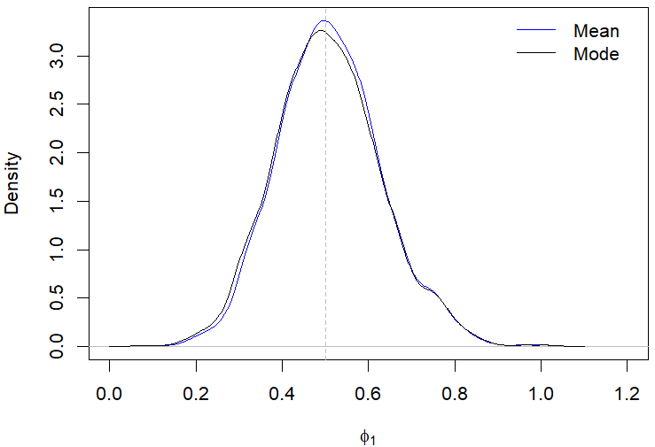 | 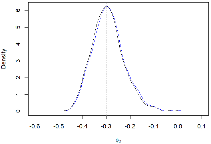 |
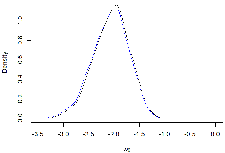
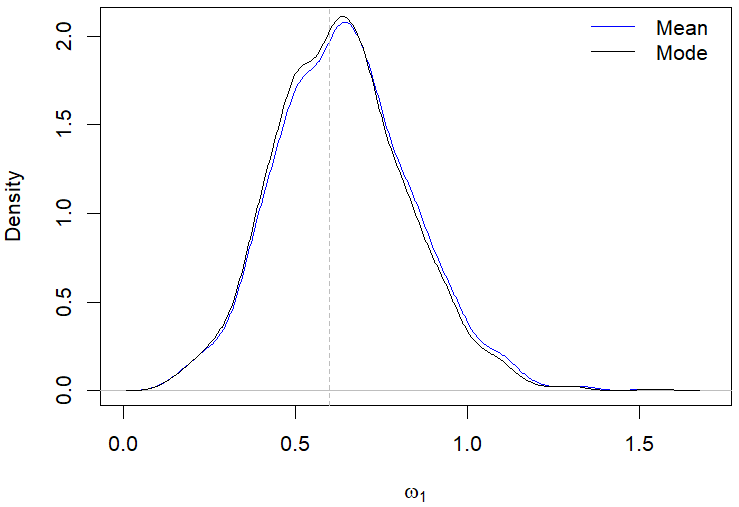
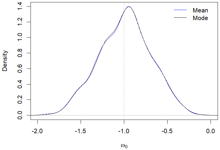
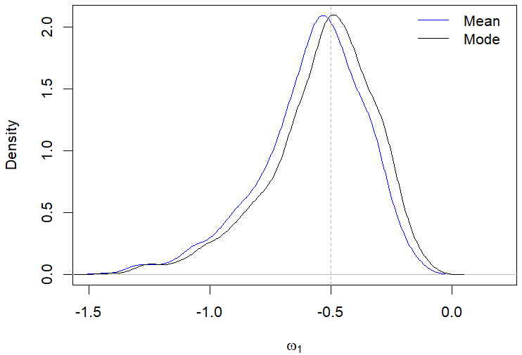
Still regarding the results displayed in Table 2, the posterior modes estimates showed a better performance compared to the posterior mean in most of the evaluated scenarios. For example, Figures 1(a)-1(d) illustrate the behavior of the posterior means and modes for a specific case in the first scenario. The only situation where the posterior mean presented a better performance than the mode was when evaluating the parameter \(\omega_0\) in the second scenario with \(n\) equal 200, which is highlighted in Table 2.
When evaluating the simulation results of the third and fourth settings, which correspond to models with seasonal patterns, we verified in Table 3 that the results of the CB were consistent with the results of configurations I and II, showing a decrease as the sample size increased.
The values of the CE approached to one, but showed an increase in two situations associated with the parameter \(\phi_1\), which are highlighted in Table 3.
| Scenario | n | \(\pmb{\theta}\) | Real | Mean | Mode | SD | CB | CE | \(\hat{R}\)-split |
|---|---|---|---|---|---|---|---|---|---|
| 150 | \(\omega_0\) | -2.000 | -2.115 | -2.085 | 0.365 | 0.153 | 1.044 | 1.001 | |
| \(\omega_1\) | 0.600 | 0.654 | 0.641 | 0.192 | 0.277 | 1.034 | 1.001 | ||
| \(\phi_1\) | 0.500 | 0.495 | 0.485 | 0.116 | 0.176 | 1.000 | 1.000 | ||
| \(\Phi_1\) | 0.500 | 0.486 | 0.478 | 0.108 | 0.165 | 1.009 | 1.000 | ||
| 200 | \(\omega_0\) | -2.000 | -2.063 | -2.043 | 0.306 | 0.129 | 1.018 | 1.001 | |
| \(\omega_1\) | 0.600 | 0.632 | 0.622 | 0.162 | 0.230 | 1.016 | 1.001 | ||
| \(\phi_1\) | 0.500 | 0.493 | 0.485 | 0.100 | 0.151 | 1.002 | 1.000 | ||
| \(\Phi_1\) | 0.500 | 0.489 | 0.483 | 0.093 | 0.141 | 1.007 | 1.000 | ||
| IV | 150 | \(\omega_0\) | -1.000 | -0.949 | -0.948 | 0.360 | 0.275 | 1.010 | 1.000 |
| \(\omega_1\) | -0.500 | -0.612 | -0.558 | 0.267 | 0.422 | 1.092 | 1.000 | ||
| \(\phi_1\) | -0.800 | -0.794 | -0.795 | 0.045 | 0.045 | 1.009 | 1.000 | ||
| \(\Phi_1\) | 0.200 | 0.201 | 0.196 | 0.074 | 0.282 | 1.000 | 1.000 | ||
| 200 | \(\omega_0\) | -1.000 | -0.988 | -0.988 | 0.311 | 0.241 | 1.000 | 1.000 | |
| \(\omega_1\) | -0.500 | -0.578 | -0.536 | 0.228 | 0.348 | 1.060 | 1.000 | ||
| \(\phi_1\) | -0.800 | -0.794 | -0.795 | 0.038 | 0.039 | 1.013 | 1.000 | ||
| \(\Phi_1\) | 0.200 | 0.201 | 0.198 | 0.063 | 0.250 | 1.000 | 1.000 |
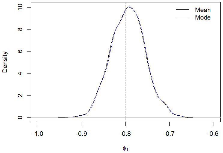
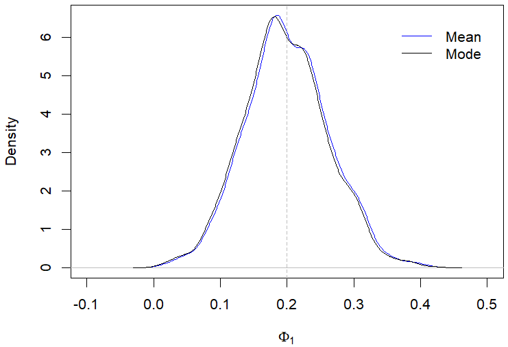
It can be observed from Table 3 that there was no significant superiority of the performance of the posterior mode estimates compared to the posterior mean estimates in scenarios III and IV. In Figures 2(a)-2(d), we illustrate the behavior of the posterior means and modes for cases of the fourth scenario. Regarding the posterior standard deviations, our results indicated a reduction in the magnitude of the deviations as the sample size increased, which also occurred in scenarios I and II.
| (a) | (b) |
 |  |
| (c) | (d) |
 |  |
Overall, the computationally results indicated good properties of inference in terms of the reduction of CB values as the sample size increased. However, we noted some alternation between the performance of the posterior mean and mode, especially in configurations III and IV.
Analysis of the influenza mortality series tuque p/
We considered data on the number of deaths, hospitalizations, and average length of hospital stay for individuals aged \(\geq\) 70 years due to influenza in the city of São Paulo, Brazil. Our data were provided by the Departamento de Informática do Sistema Único de Saúde and cover the period from January 2008 to September 2022 (Ministério, 2022).
In the studied period 97 deaths were reported, resulting in an average of 0.548 deaths per month due to influenza. However, as we can see in Figure 3(a), counts equal to zero occurred in 75.10% of the months, suggesting an excess zeros situation. When we removed the months without deaths, the monthly average was approximately two deaths. Regarding the skewness and kurtosis measures, the results indicated an asymmetric and leptokurtic behavior, as the estimated values were 4.650 and 25.124, respectively. Additionally, the sample variance was estimated at 2.374, which is approximately 4.332 times greater than the mean.
| (a) | (b) |
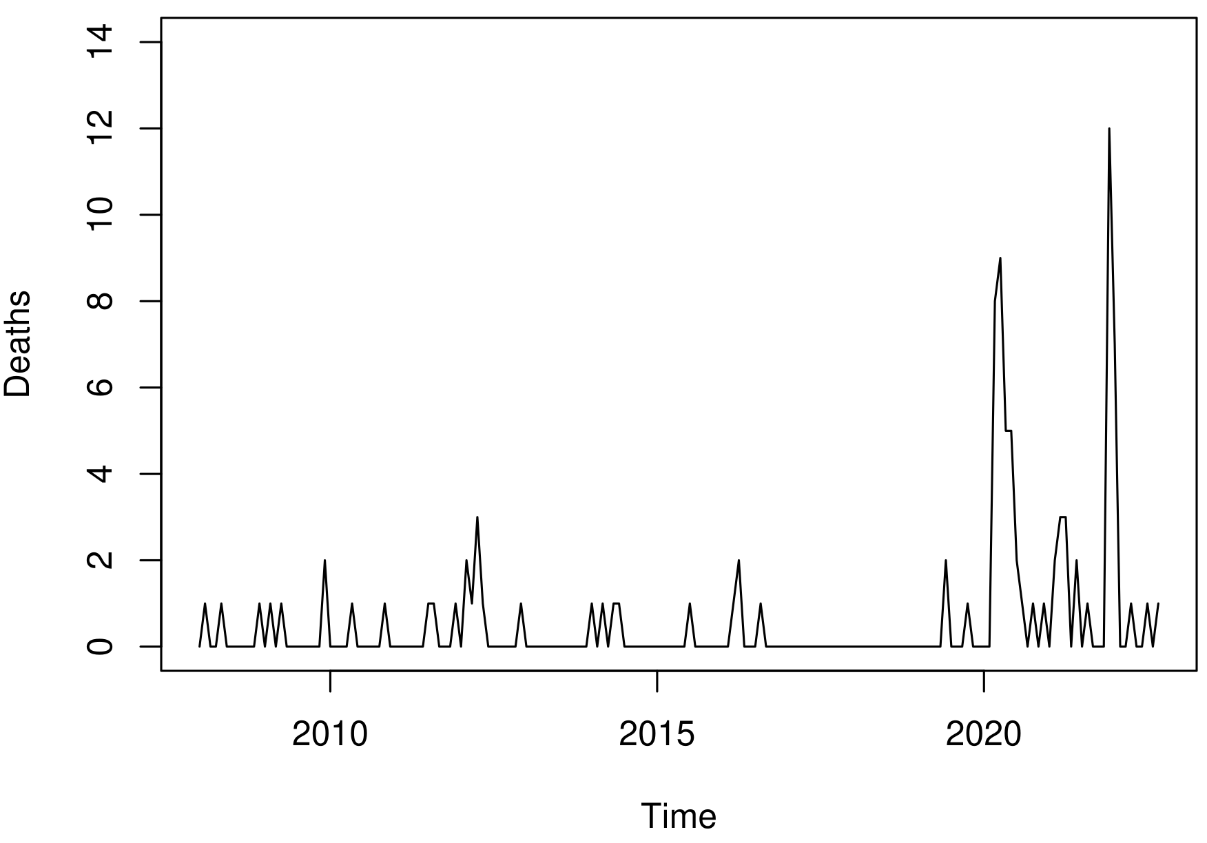 | 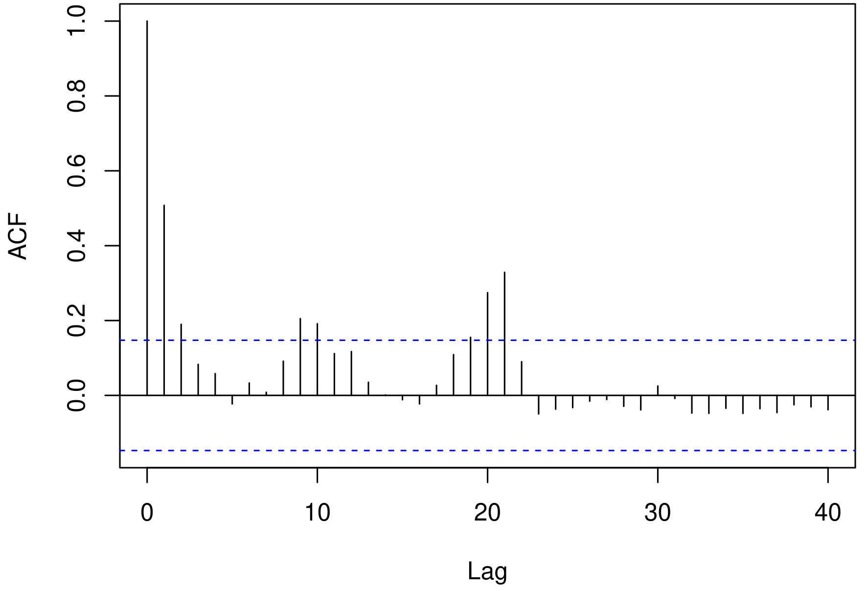 |
The behavior of the autocorrelation function (ACF) of the time series of deaths, presented in Figure 3(b), suggested a non-stationary time series. The null hypothesis of no trend was not rejected by the Cox-Stuart test (p-value = 0.405) (Cox & Stuart, 1955). Analogously, the Canova and Hansen test (Canova & Hansen, 1995) did not suggest the presence of a seasonal component (p-value = 0.402).
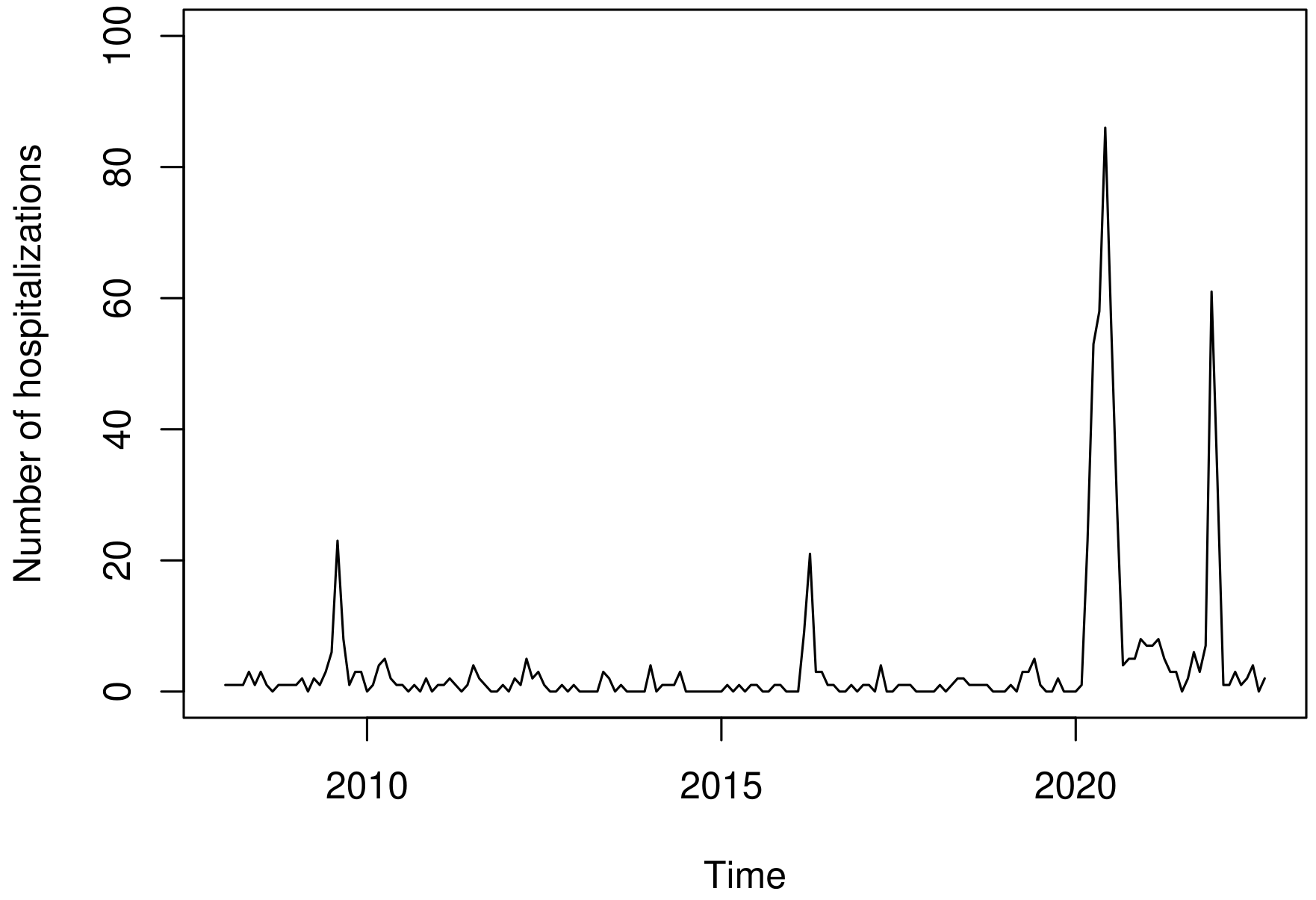
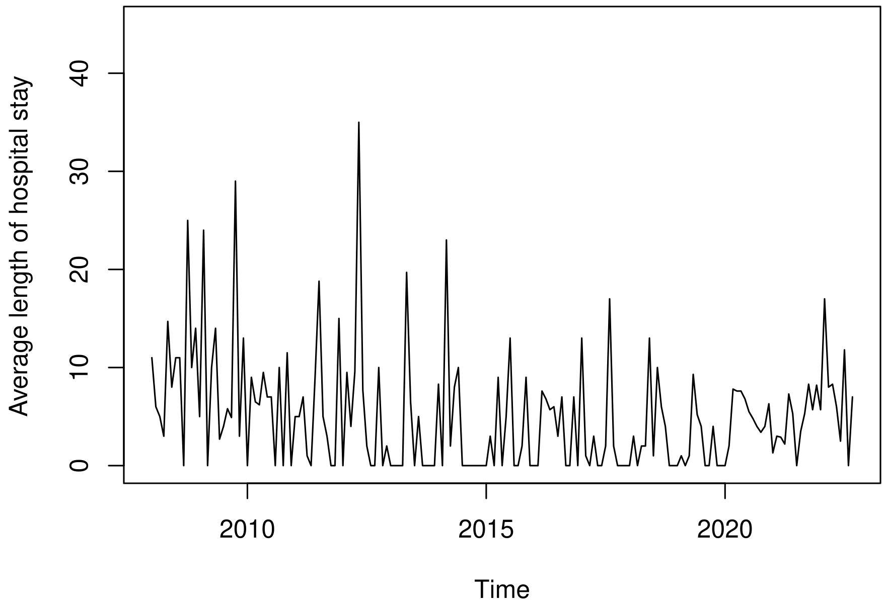
The behavior of the explanatory variables used to model the number of deaths (\(y_t\)) is shown in Figure 4. In Figure 4(a), we presented the number of hospitalizations, which show an average of approximately 4 hospitalizations per month, and in Figure 4(b) we presented the monthly average length of hospital stay. The mean of the hospitalization time was approximately 5 days, with a maximum of 35 days. According to our data, these hospitalizations resulted in an average cost of R$ 1.111,57 and a total cost of R$ 772.540,90 to the healthcare system.
For modeling the series \(y_t\), the first lag of the number of hospitalizations (\(x_{t1}\)) and the average length of hospital stay (\(x_{t2}\)) were considered as explanatory variables, arranged in \(\pmb{x}_{t}\), along with a second-order autoregressive structure. It is, we suppose that \(y_t \mid \mathcal{F}_{t-1} \sim ZAP(\mu_t, \nu_t)\), where: \[\begin{aligned} \log(\mu_t) & = (1-\phi_1B - \phi_2B^2)\left[\pmb{x}^{\top}_{t-1}\pmb{\beta} - \log(y_t)\right] + \log(y_t),\\ \nonumber logit(\nu_t) & = \omega_0 + \omega_1 y_{t-1}. \end{aligned}\]
| (a) | (b) |
 |  |
The posterior sampling was performed via HMC using 10,000 iterations, warm-up equal to 4,000, thin equal to 2, and 3 chains. According to the results, the \(\beta_2\) parameter, associated with the average length of hospital stay, was not statistically significant at a 95% credibility level, suggesting that higher average hospitalization times were not associated with an increase in deaths. Therefore, this variable was excluded from the model, and the updated results are presented in Table 4.
| Model | Parameter | Mean | SD | HPD (95%) | \(\hat{R}\)-split | ||||||
| \(L_{l}\) | \(L_{u}\) | ||||||||||
| ZAP(\(\mu_t\), \(\nu_t\)) | \(\beta_1\) | 0.018 | 0.004 | 0.009 | 0.025 | 1.000 | |||||
| \(\phi_1\) | 0.187 | 0.082 | 0.030 | 0.353 | 1.000 | ||||||
| \(\phi_2\) | -0.266 | 0.072 | -0.406 | -0.119 | 1.000 | ||||||
| \(\omega_0\) | 1.376 | 0.203 | 0.990 | 1.782 | 1.000 | ||||||
| \(\omega_1\) | -0.427 | 0.149 | -0.751 | -0.166 | 1.000 | ||||||
The \(\beta_1\) estimates indicated a positive association between the number of hospitalizations due to influenza in the period \(t-1\) and the number of deaths in the month \(t\), being statistically significant. In addition to the parameter \(\beta_1\), the parameters associated with the dependence structure, it is, \(\phi_1\) and \(\phi_2\), were also statistically significant at the same level of credibility.
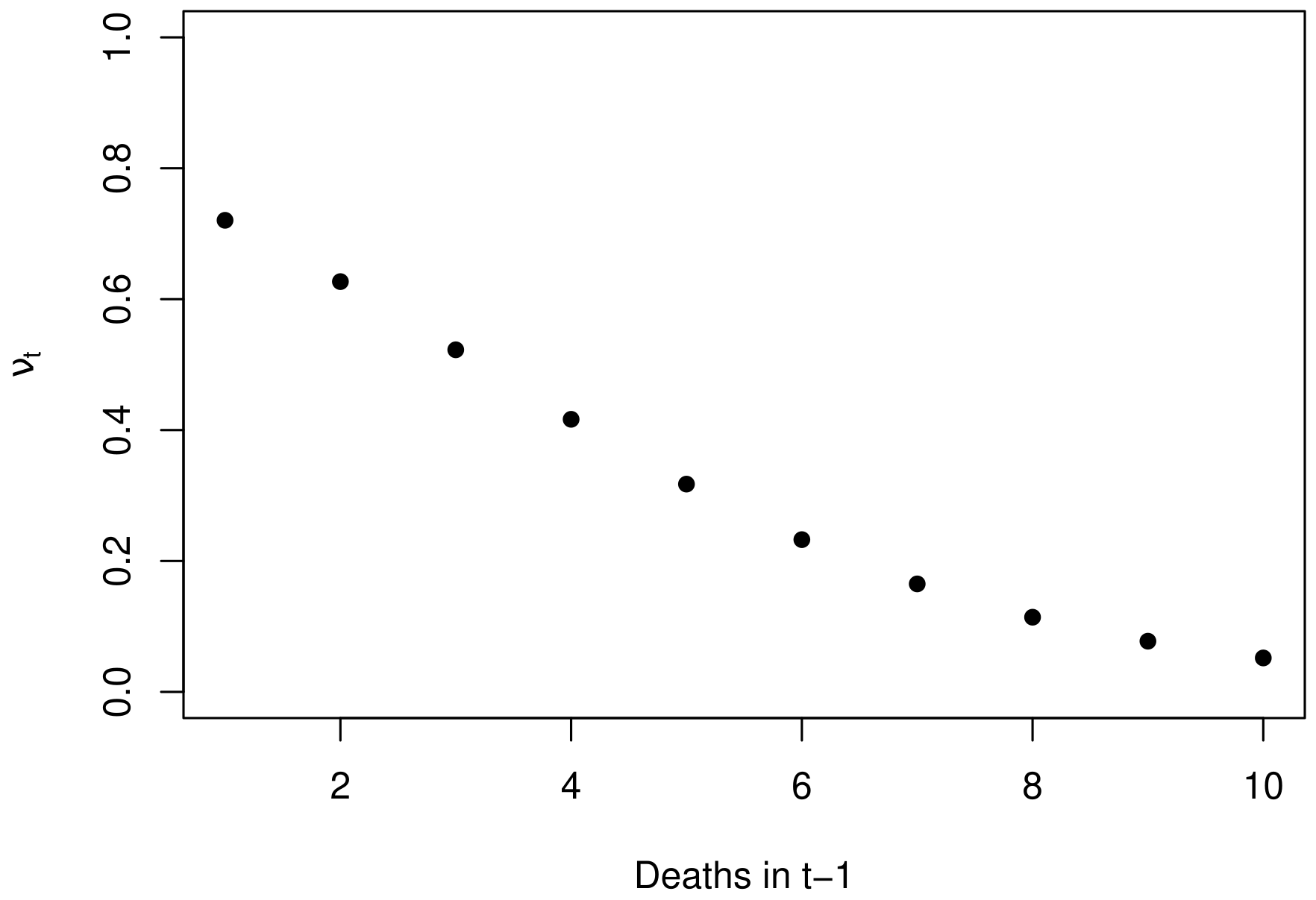
The \(\omega_0\) and \(\omega_1\) posterior estimates indicated that if there are no deaths in a given month \(t-1\), the probability of no deaths occurring in the month \(t\) is 0.798 and we can observe a reduction in this probability as the number of deaths in \(t-1\) increases. For example, if there are 5 deaths in a given month \(t-1\), the estimated probability of no deaths occurring in month \(t\) is 0.318.
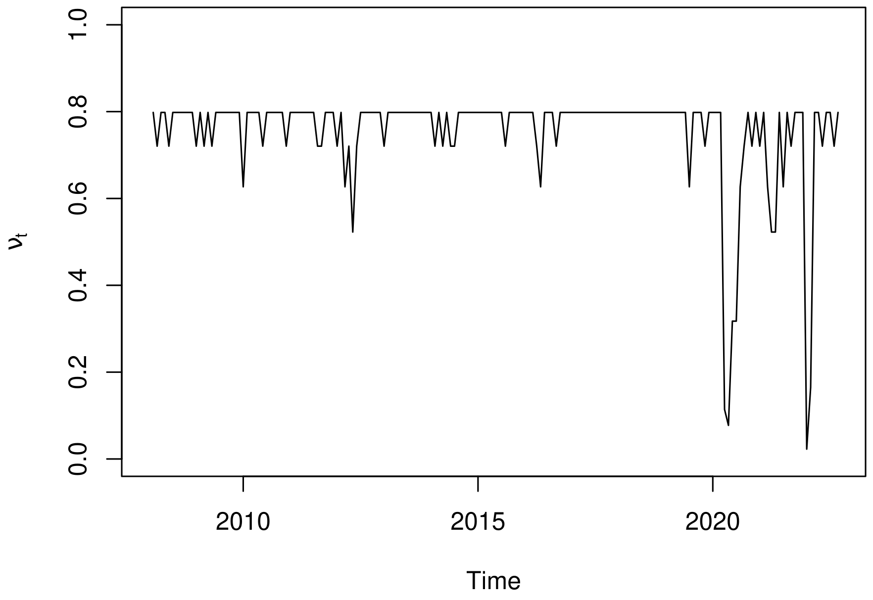
The Figure 5(a) presents the probability of the number of deaths to be zero in a month \(t\) based on the number of deaths reported in the month \(t-1\), estimated according the equation logit(\(\nu_t\)) = \(\widehat{\omega}_0 + \widehat{\omega_1} y_{t-1}\). The latent behavior of \(\nu_t\) over time is shown in Figure 5(b); note that it is possible to observe periods of reduced probability of zero deaths, such as in May 2020 and January 2022, where \(\widehat{\nu_t}\) was estimated in 0.078 and 0.023, respectively.
| (a) | (b) |
 |  |
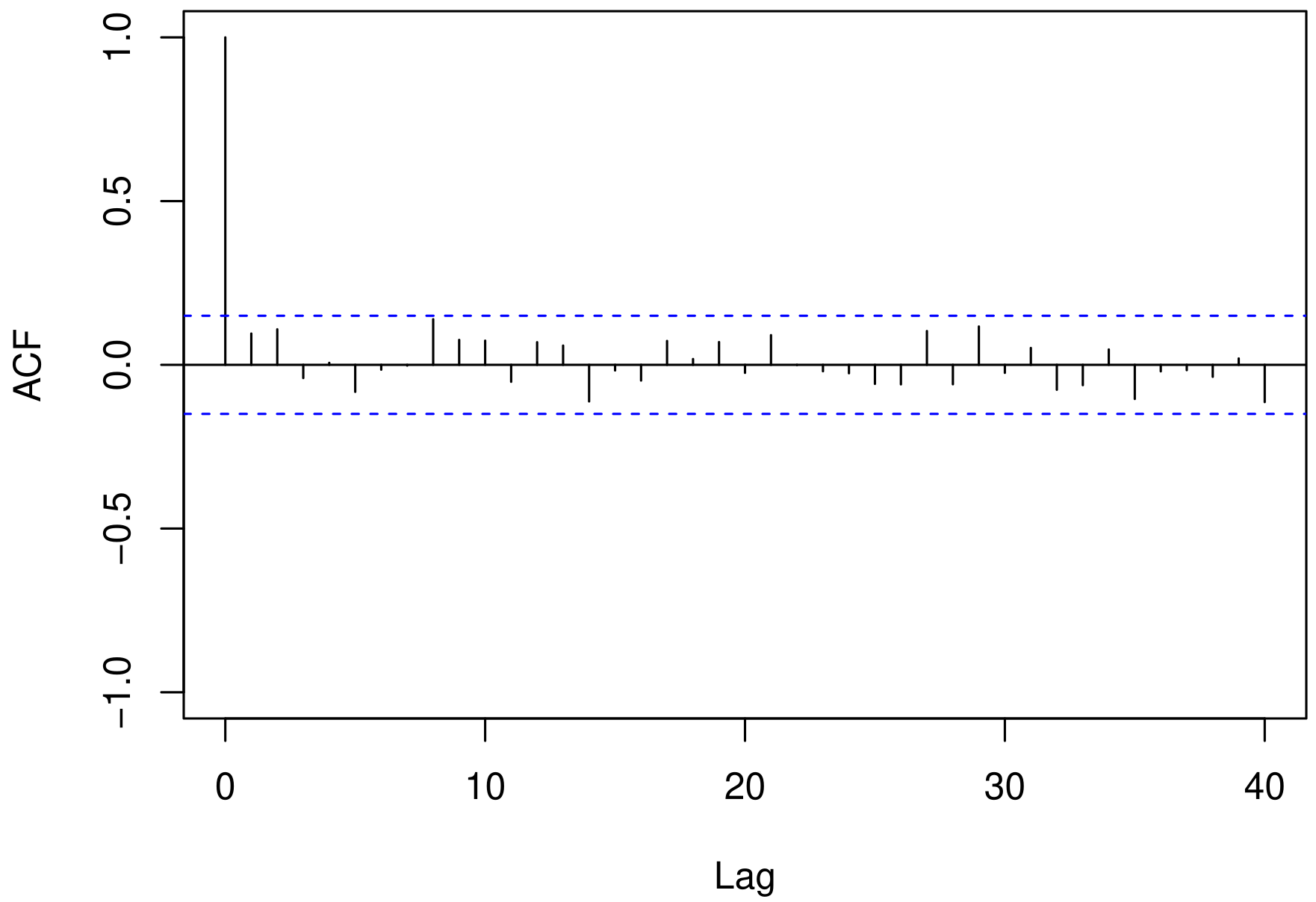
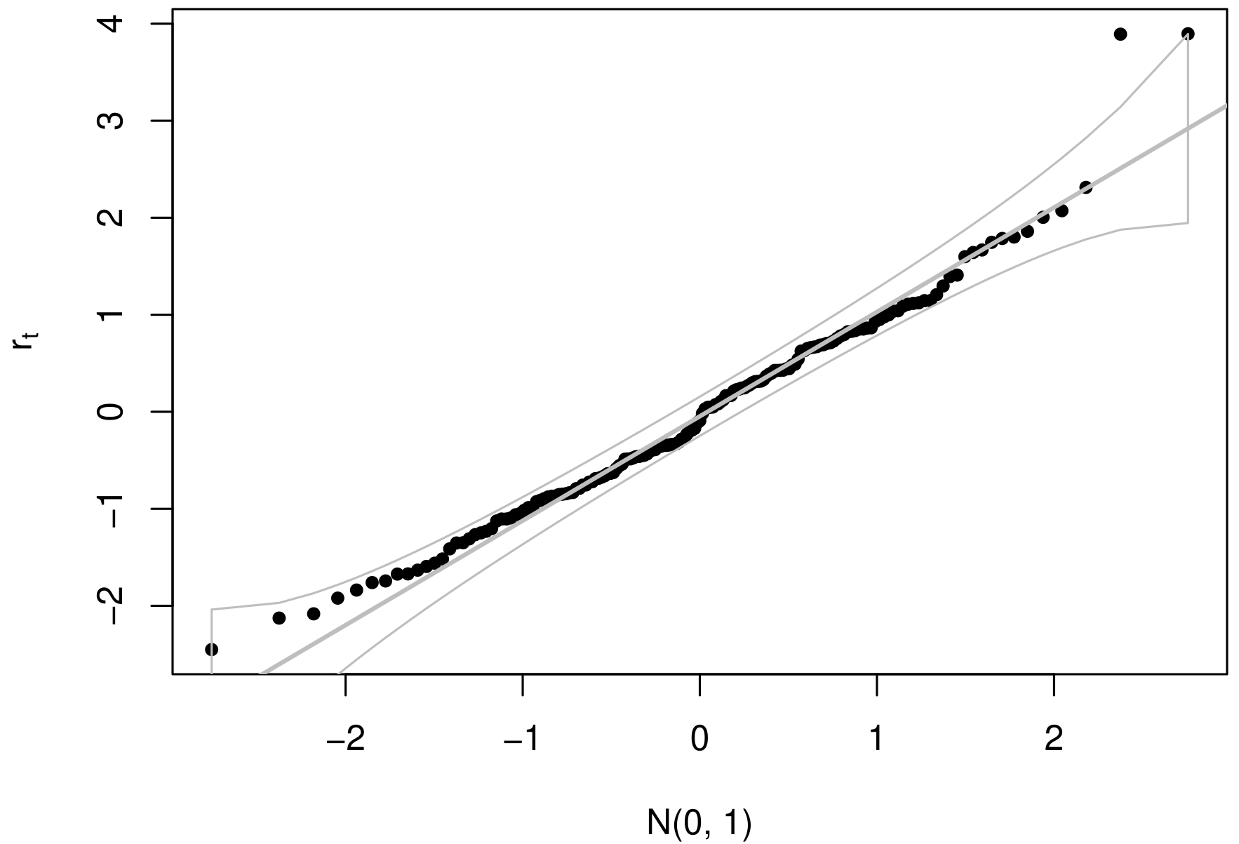
By evaluating the behavior of the normalized randomized quantile residuals (\(r_t\)) developed by Dunn & Smyth, 1996, we can observe, through Figure 6, that they exhibited an stationary behavior, as also indicated by the Box-Pierce test (Box & Pierce, 1970) evaluated up to lag 24 (p-value = 0.402). Furthermore, the null hypothesis of normality of the residuals was not rejected according to the Kolmogorov-Smirnov test (p-value = 0.776).
| (a) | (b) |
 |  |
With the verification of the stationary behavior of the residuals, we can make predictions of the number of deaths due to influenza using the expected value of the predictive distribution, estimated through Monte Carlo sampling, with parameters given by: \[\begin{aligned} \log(\mu_t) & = (1-\phi_{1}^{i}B - \phi_{2}^{i}B^2) [\beta_{1}^{i}x_{t-1,1} - \log(y_{t})] + \log(y_{t})\\ & = \beta_{1}^{i}x_{t-1,1} - \phi_{1}^{i}[\beta_{1}^{i}x_{t-2,1} - \log(y_{t-1})] - \phi_{2}^{i}[\beta_{1}^{i}x_{t-3,1} - \log(y_{t-2})],\\ logit(\nu_t) & = \omega_{0}^{i} + \omega_{1}^{i}y_{t-1}, \quad i = 1, \dots, 1000. \end{aligned}\]
The forecast for October 2022 showed that no deaths are expected, as the expected value of \(y_{oct}\) \(\approx\) 0. In the same month, the estimated probability of no deaths occurring was 0.719, with a 95% credibility interval ranging from 0.644 to 0.797. However, the expected value of the positive component, i.e., E(\(y_{oct}\mid y_{oct} > 0\)), approaches 1. This indicates that if deaths occur in October 2022, the expected count is equal to one.
Conclusion
In this paper, a GARMA(p, q) approach was proposed for modeling time series with excess zeros assuming a zero-adjusted Poisson distribution with time-varying parameters. This approach allows the evaluation and forecasting of zero counts through the parameter \(\nu_t\). We adopted a Bayesian-inference perspective using the HMC algorithm for sampling from the joint posterior, which can provide benefits in terms of exploring the parameter space.
In order to evaluate the inferential performance, a simulation study was conducted considering variations in the autoregressive orders and the proportion of zeros. The computational results indicated a good inferential performance, with improvements in most cases as the sample size increased. Regarding the application of the model to influenza data, we verified the applicability and usefulness of the model in enabling the prediction and measurement of the probability of death occurrence.
Author contributions
L. O. O. Pala participated in: Conceptualization, Data Curation, Formal Analysis, Investigation, Methodology, Programs, Writing – original draft and revision. T. Sáfadi participated in: Conceptualization, Data Curation, Formal Analysis, Investigation, Methodology, Programs, Supervision, Writing – original draft and revision.
Conflicts of interest
The authors certify that there is not a commercial or associative interest that represents a conflict of interest in relation to the manuscript.
Acknowledgments
This study was financed in part by the Coordenação de Aperfeiçoamento de Pessoal de Nível Superior - Brasil (CAPES) - Finance Code 001.
References
Stasinopoulos, M. & Rigby, R. (2020). Distributions for Generalized Additive Models for Location Scale and Shape.
Rigby, R., Stasinopoulos, M., Heller, G. & Bastiani, F. (2019). Distributions for modeling location, scale, and shape: using GAMLSS in R. Chapman & Hall.
Stan Development Team (2022). RStan: the {R.
Gelman, A., Carlin, J., Stern, H. & Rubin, D. (2014). Bayesian data analysis. Chapman & Hall.
Andrade, B., Andrade, M. & Ehlers, R. (2015). Bayesian GARMA models for count data. 1(4), 192-205. https://doi.org/10.1080/23737484.2016.1190307
Maiti, Raju, Biswas, Atanu & Chakraborty, Bibhas (2018). Modelling of low count heavy tailed time series data consisting large number of zeros and ones. 27(3), 407–435. https://doi.org/10.1007/s10260-017-0413-z
Ministério da Saúde (2022). Morbidade hospitalar do Sistema Único de Saúde.
Duane, S., Kennedy, A., Pendleton, B. & Roweth, D. (1987). Hybrid Monte Carlo. 195(2), 216-222. https://doi.org/10.1016/0370-2693(87)91197-X
McElreath, R. (2020). Statistical Rethinking: A Bayesian Course with Examples in R and Stan. Chapman & Hall.
Burda, M. & Maheu, J. (2013). Bayesian adaptive Hamiltonian Monte Carlo with an application to high-dimensional BEKK GARCH models. 345-372.
Conceicao, K., Suzuki, A. & Andrade, M. (2021). A Bayesian approach for zero-modified Skellam model with Hamiltonian MCMC. 30(2), 747-765. https://doi.org/10.1007/s10260-020-00541-7
Benjamin, M., Rigby, R. & Stasinopoulos, M. (2003). Generalized Autoregressive Moving Average Models. 98(461), 214-223. https://doi.org/10.1198/016214503388619238
Rocha, A. V. & Cribari-Neto, F. (2008). Beta autoregressive moving average models. 18(3), 529-545. https://doi.org/10.1007/s11749-008-0112-z
Hoffman, M. & Gelman, A. (2014). The No-U-Turn Sampler: Adaptively Setting Path Lengths in Hamiltonian Monte Carlo. 15(1), 1593-1623. https://doi.org/10.48550/arXiv.1111.4246
Broemeling, L. (2019). Bayesian analysis of time series. CRC Press.
Safadi, T. & Morettin, P. (2003). A Bayesian analysis of autoregressive models with random normal coefficients. 73(8), 563-573. https://doi.org/10.1080/0094965031000136003
Khandelwal, I., Adhikari, R. & Verma, G. (2015). Time series forecasting using hybrid ARIMA and ANN models based on DWT decomposition. 173-179. https://doi.org/10.1016/j.procs.2015.04.167
Box, G. & Jenkins, G. (1976). Time series analysis, forecasting and control. Holden-Day.
Silva, R. (2020). Generalized Autoregressive Neural Network Models. https://doi.org/10.48550/arXiv.2002.05676
Bayer, F., Cintra, R. & Cribari-Neto, F. (2018). Beta seasonal autoregressive moving average models. 88(15), 2961-2981. https://doi.org/10.1080/00949655.2018.1491974
Davis, R., Fokianos, K., Holan, S., Joe, H., Livsey, J., Lund, R., Pipiras, V. & Ravishanker, N. (2021). Count time series: A methodological review. 116(55), 1533-1547. https://doi.org/10.1080/01621459.2021.1904957
Sales, L., Alencar, A. & Ho, L. (2022). The BerG generalized autoregressive moving average model for count time series. 1-13. https://doi.org/10.1016/j.cie.2022.108104
Barreto-Souza, W. (2017). Mixed Poisson INAR(1) processes. 2119–2139. https://doi.org/s00362-017-0912-x
Ghahramani, M & White, SS (2020). Time Series Regression for Zero-Inflated and Overdispersed Count Data: A Functional Response Model Approach. 14(2), 1-18. https://doi.org/10.1007/s42519-020-00094-8
Payne, E., Hardin, J., Egede, L., Ramakrishnan, V., Selassie, A. & Gebregziabher, M. (2017). Approaches for dealing with various sources of overdispersion in modeling count data: Scale adjustment versus modeling. 26(4), 1802-1823. https://doi.org/10.1177/0962280215588
Briet, O., Amerasinghe, P. & Vounatsou, P. (2013). Generalized Seasonal Autoregressive Integrated Moving Average Models for Count Data with Application to Malaria Time Series with Low Case Numbers. 8(6), 1-9. https://doi.org/10.1371/journal.pone.0065761
Alqawba, M., Diawara, N. & Chaganty, N. (2019). Zero-inflated count time series models using Gaussian copula. 38(3), 342-357. https://doi.org/10.1080/07474946.2019.1648922
Tawiah, K., Iddrisu, W. & Asosega, K. (2021). Zero-Inflated Time Series Modelling of COVID-19 Deaths in Ghana. 1-9.
Melo, M. & Alencar, A. (2020). Conway–Maxwell–Poisson Autoregressive Moving Average Model for Equidispersed, Underdispersed, and Overdispersed Count Data. 41(6), 830-857.
Feng, C. (2021). A comparison of zero-inflated and hurdle models for modeling zero-inflated count data. 8(1), 1-19. https://doi.org/10.1186/s40488-021-00121-4
Aragaw, A., Azene, A. & Workie, M. (2022). Poisson logit hurdle model with associated factors of perinatal mortality in Ethiopia. 9(16), 1-11. https://doi.org/10.1186/s40537-022-00567-6
Hashim, L., Hashim, K. & Shiker, M. (2021). An Application Comparison of Two Poisson Models on Zero Count Data. https://doi.org/10.1088/1742-6596/1818/1/012165
Tian, G., Liu, Y., Tang, M. & Jiang, X. (2018). Type I multivariate zero-truncated/adjusted Poisson distributions with applications. 132-153. https://doi.org/10.1016/j.cam.2018.05.014
Box, G. & Pierce, D. (1970). Distribution of Residual Autocorrelations in Autoregressive-Integrated Moving Average Time Series Models. 65(332), 1509-1526. https://doi.org/10.1080/01621459.1970.10481180
Cox, D. & Stuart, A. (1955). Some Quick Sign Tests for Trend in Location and Dispersion. 42(1), 80-95. https://doi.org/10.2307/2333424
Canova, F. & Hansen, B. (1995). Are Seasonal Patterns Constant over Time? A Test for Seasonal Stability. 13(3), 237–252. https://doi.org/10.2307/1392184
R Core Team (2022). R: A Language and Environment for Statistical Computing.
Dunn, P. & Smyth, G. (1996). Randomized Quantile Residuals. 5(3), 236-244. https://doi.org/10.2307/1390802
Neal, R. (2011). MCMC using Hamiltonian dynamics. Chapman & Hall. 1-51.
Ehlers, R. (2019). A Conway-Maxwell-Poisson GARMA Model for Count Data. 1-11.
Mikis Stasinopoulos, Bob Rigby & Paul Eilers (2016). gamlss.util: GAMLSS utilities.
Zuur, A., Ieno, E., Walker, N., Saveliev, A. & Smith, G. (2009). Mixed effects models and extensions in ecology with R.. Springer.
Bertoli, Wesley, Conceição, Katiane S., Andrade, Marinho G. & Louzada, Francisco (2021). A New Regression Model for the Analysis of Overdispersed and Zero-Modified Count Data. 23(646), 1-25. https://doi.org/10.3390/e23060646