Three-Dimensional Modeling of Faces Utilizing Robust Characteristics
DOI 10.5433/1679-0375.2024.v45.48505
Citation Semin., Ciênc. Exatas Tecnol. 2024, v. 45: e48505
Received: 19 August 2023 Received in revised for: 2 May 2024 Accepted: 24 June 2024 Available online: 7 August 2024
Abstract:
The modeling of human faces is an integral part of a variety of computer applications, from animation and entertainment programs to security and facial recognition apps. This paper presents an alternative method that, given a photo as input, extracts a set of landmarks, anatomical points extracted from a human’s face, modifying a triangular polygonal mesh using principles of computer graphics so that it resembles the face whose characteristics have been extracted without requiring additional input from the user. After the creation of the initial mesh, this method, implemented in Python for testing purposes, utilizes principles of three-dimensional mesh modeling such as the use of delta-coordinates to allow the user to perform controlled modifications in the mesh by moving the landmarks. The meshes generated by this method maintain the format and colors of the original face, extracted from the photo offered as input, with tests showing the resistance of the mesh to deformation, as well as corroborating that there is little to no effect on the speed of how modifications are performed based on the degree of the vertex or by how much it is moved.
Keywords: three-dimensional modeling, human faces, landmarks, points, computer graphics
Introduction
Polygonal meshes are a versatile tool of computer graphics, allowing a bidirectional non-oriented graph to describe a geometric form through the position of its vertices and their connections, as described in Botsch et al., 2007.
One form that can be described by polygonal meshes is the human face. Facial Modeling serves as the basis for various applications, from facial recognition and reconstruction according to Kittler et al., 2016, to artistic rendering or the creation of avatars in social applications. Some applications can create a set of three-dimensional models based on two-dimensional images. For example, in a study by Afzal et al., 2020 they were able to extract characteristics and depth data to generate a set of three-dimensional images from a single original image.
Anatomical traits such as the size, shape and arrangement of common features, such as the eyes, nose and mouth, ensure that the face of two different humans will differ between each other ([RICHMOND - missing information]). Consequently, the facial meshes generated from these faces will also differ. However, using techniques such as linear differential coordinates and the continuous Laplace–Beltrami operator (Lipman et al., 2004; Sorkine, 2006), we are able to alter the positions of the vertices without changing the existing edges (Soares, 2007). This way, a basic mesh with a preset layout of edges can be used to, after modeling the features unique to each person, singularly represent each of these different people.
The Laplace-Beltrami operator enables the smooth propagation of changes made to a vertex to its neighbors, allowing users to modify a mesh without altering the configuration of neighboring points. The resulting changes differ from what might happen if an point-cloud based algorithm (Xian-Feng et al., 2017) is used, as point-clouds are groups of points in space with no edges between them and instead each point of the cloud represents a measurement on a object’s surface.
Likewise, the use of a generic face model that is morphed to adapt to a sample can be seen in studies such as the one performed by Ansari A-Nasser et al., 2009 where a generic model is aligned with a image for duplication using three points. The triangular mesh model is then deformed using data from features extracted from the sample to improve similarity to the original. This technique can be expanded to the whole human body, as shown by Zhang & Xiao, 2021 creating a three-dimensional mesh of a body based on a single image using flexible mesh deformation, going so far as to include details of the clothes being worn in the sample pictures. Allowing generic models to morph into any specific face means that input can be standardized.
We propose a method that combines elements of these different approaches to mesh editing. Given a photo of a human face used as input, extracts features from this photo to generate a triangular polygonal mesh of the face while maintaining color information. Afterwards, modifications can be performed on the position of any individual vertex, which will be distributed to neighboring vertices while maintaining the structural integrity of the mesh. After these changes, the effect on adjacent points is calculated, and a new version of the mesh will be created, reflecting those changes.
After implementing the proposed method, we test the robustness of the meshes, the speed of the creation process, and the calculations after moving a vertex and if the new mesh has peculiar deformations that are not smoothed among neighbors, as any peaks on a face without a gradual rise would be unnatural.
In the following, we describe the implementation of the proposed method in Materials and methods, Discuss the results, and finally present our Conclusions.
Material and methods
The proposed method is divided in four main steps, as shown in the flowchart presented in Figure 1.

First, we extract landmark data from a photo used as input by the user. Obtaining this data, we create a triangular mesh by using the position and color information of these points. After the mesh has been created, we allow the user to modify any given vertex in the mesh by giving it an offset from its current position in the \(x\), \(y\) and \(z\) axes. If a vertex is edited, we recreate the mesh by adjusting the position of the vertex and adjusting the rest of the mesh, and the user may then edit another vertex.
For the purposes of the method, let \(\mathbf{M = (V, E, F)}\) be a polygonal mesh described by \(\mathbf{V}\), a set of vertices in three dimensional space; \(\mathbf{E}\), a set of edges between the members of \(\mathbf{V}\) and \(\mathbf{F}\), the set of faces of \(\mathbf{M}\) described by \(\mathbf{V}\) and \(\mathbf{E}\). \(\mathbf{M}\) can be categorized by the shapes of \(\mathbf{F}\). For example, if the shapes are triangles, the mesh is a triangular mesh.
Mesh creation
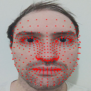
The only material required for the initial step of the proposed method is a photo of a human face. With the tools available in MediaPipe “Face Mesh” (Google, 2019), we are able to extract a set of 468 relevant three-dimensional landmarks from the photo as seen in Figure 2.

The landmarks, shown in Figure 2 as red dots, have a position in the \(x\) and \(y\) axis between 0 and 1, similar to the corners of a square of area 1. The position on the \(z\) axis, however, is negative, as the origin of the system is at the point where the digital camera which is used to infer depth from the two-dimensional photo is positioned. These positions are inferred through the use of two deep learning neural networks that work in tandem: one detects the landmarks on the face, while the other predicts the three-dimensional surface of the face, even if it is not completely visible. With the coordinates for all vertices in three-dimensional space, we shall use these 468 points as our \(\mathbf{V}\) set. Algorithm [alg:landmark_extraction] details how landmarks are extracted from a photo.
Algorithm 1: Landmark Extraction
        1: function landmarkExtraction(path)

        2: Initialize: vx, vy, vz, V , colordata

        3: Import libraries for face mesh detection

        4: face_mesh <- FaceMesh(static_image_mode=True)

        5: img <- image read from path

        6: get img width and height

        7: get pixel_values from img

        8: results <- img processed using face_mesh with RGB conversion

        9: landmarks <- results.landmarks

        10: for each landmark in landmarks do:

        11: x = get x-coordinate of the landmark

        12: y = get y-coordinate of the landmark

        13: z = get z-coordinate of the landmark

        14: append x to vx; y to vy; z to vz and [x, y, z] to V list

        15: relative_x = calculate relative x-coordinate within the image

        16: relative_y = calculate relative y-coordinate within the image

        17: append pixel value at (relative_x, relative_y) to colordata list

        18: end for

        19: return landmarks, vx, vy, vz, colordata, V

        20: end function
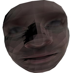
Using the edge list provided by Face Mesh as our set \(\mathbf{E}\), along with RGB color information extracted from the pixels occupied by the landmarks in the photo, we can color the new mesh according to the input. We are able to create a mesh \(\mathbf{M}\) based on the face in the photo, as shown in Figure 3, by first calculating the members of set \(\mathbf{F}\), which will remain static regardless of how many times the mesh might be modified, and then using the current spatial information of set \(\mathbf{V}\) alongside the color data extracted from the photo.

Mesh editing
After the creation of the mesh \(\mathbf{M}\), the user is allowed to modify the position in three-dimensional space of any given vertex of \(\mathbf{V}\). To allow this process to happen without severing the edges of \(\mathbf{E}\), we use the Laplace-Beltrami operator, a differential second order operator defined as the divergence of the gradient of a function. In Euclidean space, the Laplacian is given by the sum of the pure second derivatives of the function in respect to each of the independent variables, allowing operations defined in sub-varieties in Euclidean space (Sorkine, 2006).
The Differential Coordinate, also called a \(\delta\)-coordinate, of a given vertex \(\mathbf{v}_i\) of \(\mathbf{V}\), is defined as the difference between the Cartesian coordinate of \(\mathbf{v}_i\) and the center of mass of its immediate neighbors, \(\mathbf{v}_j\).
The formula for the \(\delta\)-coordinates of a given \(\mathbf{v}_i\), in terms of the number of \(\mathbf{N}_j\) of neighbors j of vertex i and the Cartesian coordinates of each of its neighbors \(\mathbf{v}_j\) (Sorkine, 2006), is given by equation [eq_coordif]:
\[ \mathbf{\delta}_i = (\mathbf{\delta}_i(x), \mathbf{\delta}_i(y), \mathbf{\delta}_i(z)) = {v_i} - \frac{1}{N_j} \sum_{j \in N(i)} \mathbf{v}_j,\]
where \(\mathbf{\delta}_i\) are the delta-coordinates of \(\mathbf{v}_i\), \(\mathbf{\delta}_i(x)\), \(\mathbf{\delta}_i(y)\) and \(\mathbf{\delta}_i(z)\) are each of its axes and \(\sum_{j \in N(i)}\) is the sum of the neighbors of \(\mathbf{v}_i\).
As the mesh \(\mathbf{M}\) is the piecewise-linear approximation of a smooth surface (i.e. a human face), we can consider the \(\delta\)-coordinates as the discretization of the Laplace-Beltrami operator. Based on that, we can rewrite the \(\delta\)-coordinate vector as given in equation [vet_coordif]:
\[ \mathbf{\delta}_i = \frac{1}{N_j} \sum_{j \in N(i)} (\mathbf{v_i} - \mathbf{v}_j).\]
The transformation of the vector of Cartesian coordinates into the \(\delta\)-coordinates vector can be represented in matrix form. Given \(\mathbf{Adj}\) the adjacency matrix of \(\mathbf{M}\), a square matrix of \(n \times n\) elements in which each cell \(\mathbf{Adj}_{ij}\) of the matrix has a value of 1 if there is an edge in \(\mathbf{E}\) that connects vertex \(i\) to vertex \(j\), or 0 otherwise. Naturally, the main diagonal of \(\mathbf{Adj}\) is composed by zeros as a vertex cannot be its own neighbor.
Next, we define the diagonal matrix \(\mathbf{D}\) in which each element of \(\mathbf{D}_{ii}\) is the degree of the vertex \(i\), that is, the number of neighbors that vertex has. The matrix \(\mathbf{L}\), which represents the transformation matrix of Cartesian coordinates to differential coordinates is given by equation [mat_L]:
\[ \mathbf{L} = \mathbf{I} - \mathbf{D}^{-1} \mathbf{Adj},\]
where \(\mathbf{I}\) is the identity matrix, \(\mathbf{D^{-1}}\) is the inverse of matrix \(\mathbf{D}\) and \(\mathbf{Adj}\) is the adjacency matrix. The topological Laplacian of the \(\mathbf{M}\) mesh is the symmetrical version of \(\mathbf{L}\), \(\mathbf{Ls}\), which is simpler to calculate than \(\mathbf{L}\). Equation [mat_Ls] gives the formula for \(\mathbf{Ls}\)
\[ \mathbf{Ls} = \mathbf{D} - \mathbf{Adj}.\]
As such, each cell can be calculated as \(\mathbf{Ls}_{ij} = \mathbf{N}_j\), if \(i\) = \(j\), \(\mathbf{Ls}_{ij}\) = -1, if there is an edge between \(i\) e \(j\), and \(\mathbf{Ls}_{ij}\) = 0 otherwise.
From the topological Laplacian, the \(\delta\)-coordinates can be obtained from the Cartesian coordinates by multiplying \(\mathbf{Ls}\) by each of the three dimensions of the mesh \(\mathbf{M}\), e.g. the \(x\) coordinate in equation [vet_deltax]:
\[ \mathbf{Ls} x = \mathbf{\delta}(x).\]
After performing the desired transformations, it is necessary to convert the \(\delta\)-coordinates back into Cartesian coordinates. However, it is not possible to simply perform the inverse procedure as \(x\) = \(\mathbf{Ls}^{-1}{\delta}(x)\) is undefined, same for the \(y\) and \(z\) axis. This happens because both \(\mathbf{L}\) and \(\mathbf{Ls}\) are singular and the differential coordinates are invariant to translation. To perform the transformation, it is necessary to fix the position of one or more vertices that will serve as anchors. We append the identity matrix of these anchors to \(\mathbf{Ls}\), creating \(\overline{L}\), and append the absolute position of these anchors to the end of the vector of \(\delta\)-coordinates in such a way that for each axis the equation [mat_Lbarx] describes (e.g. the \(x\) axis):
\[ \overline{L} x = (\mathbf{\delta}(x) \cdot c(x)'),\]
where \(x\) is the vector that has the new positions in the \(x\) axis of Cartesian space and \({\delta}(x) \cdot c(x)'\) is the concatenation of \({\delta}(x)\) with the transposed vector containing the absolute position of the anchors in the \(x\) axis.
Finally, we append the vertex we are editing, both its identity to \(\overline{L}\) and its new position to the \(\delta\)-coordinate vector, such as the final equation [edit_x] that must be solved for each axis in editing is
\[ (Ls \cdot {I}_c \cdot {I}_e) x = (\delta(x) \cdot c(x)’ \cdot e(x)’),\] where \(Ls \cdot {I}_c \cdot {I}_e\) are \({I}_c\) and \({I}_e\) appended to \(Ls\) and \(e(x)’\) is the transposed position of the edited vertex. This yields the new positions in Cartesian space of the vertices. The use of \(\delta\)-coordinates allows the quick and robust editing of the mesh, resisting deformation and maintaining our \(\mathbf{E}\) set without requiring new edges or breaking old ones. Algorithm [alg:mesh_ed] details the mesh editing process.
Algorithm 2: Mesh Editing
        1: function find_vector(matrix, target_vector)

        2: Compute pseudoinverse of matrix

        3: solution <- pseudoinverse × target_vector

        4: return solution

        5: end function

        6: function meshEdit(V, editvertex, editoffset)

        7: initialize newx, newy and newz

        8: get x, y and z by extracting each axis of V

        9: δ(x) <- Ls · x

        10: δ(y) <- Ls · y

        11: δ(z) <- Ls · z

        12: randomly select two distinct anchors, anchor1 and anchor2 for editvertex

        13: create b, an indicator vector for anchor1

        14: create c, an indicator vector for anchor2

        15: create e, an indicator vector for editvertex

        16: L <- [Ls b c e]

        17: append all three of anchor1, anchor2, and editvertex positions to each of δ(x), δ(y), δ(z)

        18: Find newx, newy and newz:

        19: newx = find_vector(¯L, δ(x))

        20: newy = find_vector(¯L, δ(y))

        21: newz = find_vector(¯L, δ(z))

        22: return newx, newy, newz

        23: end function
Results and discussion
During testing, the steps followed were: first, a photo of a human face was supplied, so that the landmarks could be extracted and the initial mesh generated. Second, a series of modifications were performed on vertices in the mesh, with the time needed for matrix operations recorded to verify which factors could impact them.
During each test, three vertices were randomly chosen, however, each was from a specific pool, determined by their degree. First, a vertex of degree 3, the smallest degree in the mesh. Second, a vertex of degree 6, the mode of the mesh. And finally, a vertex of degree 8, the maximum of the mesh.
A picture of the author was used as input, which returned an initial mesh, as shown in the example of Figures 2 and 3. The extraction of landmarks from the photo as well as the initial modeling of the mesh were both individually timed across tests.
Afterwards, the process of editing the mesh through the use of \(\delta\)-coordinates is used six times. During the first three edits a lesser value is used compared to the second round of edits, with an offset given of (\(-0.005\), \(-0.005\), \(-0.005\)). These values have been chosen arbitrarily and are rather tame as, in the \(x\) and \(y\) axes, 0 corresponds to minimum width or height and 1 corresponds to the maximum, while for the \(z\) axis it corresponds to the distance to the virtual camera, with a lesser number being further away.
As edits stack on top of one another, these changes are performed sequentially, with a mesh being recreated from the edited vertices at the end of the third edit, performed on the vertex of degree 8.
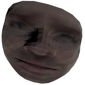
Figure 4 shows the mesh from Figure 3 after these minor edits. Albeit the mesh has been edited, to the naked eye it might be hard to detect changes to the mesh as it resists the deformation and keeps the same basic shape. As such, a second battery of edits is performed on the same vertices, both to test if there are issues performing edits on the same vertices repeatedly as well as to make more drastic changes to the mesh, to serve as an illustration to these edits.

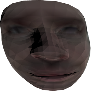
Once again the same three vertices are edited, however, instead of the previous values of (\(-0.005\), \(-0.005\), \(-0.005\)), a value of (\(0.1\), \(0.1\), \(-0.1\)) is given to each vertex. These changes, while still discretionary, are about 20 times greater than the previous edit, which, as a result, have a greater effect on the mesh. These can be seen in Figure 5.

All six edits performed during each test were individually timed as well, to see if the degree of the vertex or the amount it is edited has any impact on the processing time of the matrix operations. These results, alongside the previously recorded times, are compiled for two reference tests, labeled Test 1 and Test 2 in Table 1.
| Task | Test 1 time (s) | Test 2 time (s) |
|---|---|---|
| Landmark Extract | 0.218 | 0.214 |
| Initial Generation | 0.003 | 0.007 |
| Degree 3 edit | 0.399 | 0.362 |
| Degree 6 edit | 0.364 | 0.389 |
| Degree 8 edit | 0.366 | 0.401 |
| 2nd Degree 3 edit | 0.393 | 0.363 |
| 2nd Degree 6 edit | 0.387 | 0.374 |
| 2nd Degree 8 edit | 0.384 | 0.584 |
Discussion
Of the mesh images from test one, Figure 5 in particular illustrates how the meshes resist deformation. Instead of each of the three vertices spiking out from the mesh, their neighbors are dragged along with them, giving both the mouth and the nose a lopsided appearance.
Additionally, the Table 1 results show that, regardless of the degree of the vertex or the displacement generated by the edit, edits take on average between 0.35 seconds to 0.4 seconds. The one outlying result, the second edit of the degree eight vertex of the second test, being a result of a lag spike in the simulator. Even in results that did not experience any abnormal activity, there were no clear trends like a vertex with a higher degree taking more or less time to be edited or smaller edits being processed faster.
It should be noted that the created meshes can be placed and moved in a scene with a directed source of light, and thus intensity of color and rotation are both freely manipulated.
One thing that should be noted is that the original layout of landmarks around the human face has a distinct oval shape. However, as both the canonical model used to create the mesh is round and the mesh itself is bounded in a square around the \(x\) and \(y\) axes, the mesh ends up taking a rounded shape. This is a constraint of the implementation, not of the method itself.
Regardless, the implementation of the method has found some issues which can be improved upon, such as changing the shape of the base mesh to a more oval shape, increasing the number of vertices on the mesh to improve resolution.
Although it was not the focus of the research, the implementation of a basic user interface might help users interact with landmarks dynamically, instead of having to send offset values to a vertex in the mesh.
As for the method itself, there are some possible venues for future research, such as the creation of a vertical symmetry axis by pairing certain landmarks together, such that when a feature is edited in one side of the face, changes will be mirrored on the other side of the face.
Likewise, by comparing the length of the edges of set \(\mathbf{E}\), we can assign weights to edges based on the distance between neighbors, altering equation [vet_coordif]. This would allow neighbors of the same vertex to be affected differently by changes on that given vertex, depending on how close they are. For example, if the very tip of the nose were to be modified, a landmark closer to the tip of the nose might be more affected by a change than one at the upper lip. These weights can be modeled using static weights values, increased weight by degree of the vertex or by considering the distance between two vertices at the start of the editing process.
Conclusions
The meshes generated by the proposed method provide an alternative for spreading modifications across a mesh when a landmark in the face is modified. The number of connected landmarks allow the user to study how small changes in one or several vertices compound to move facial structures such as the mouth or nose. These meshes preserve their original edges and resist deformations due to the characteristics of the \(\delta\)-coordinates. Changes are spread across the surface of the mesh from any chosen vertex, with the speed at which the calculations are performed being unaffected by the intensity of the change or by the chosen vertex’s degree. The matrix \(\mathbf{D}\) and \(\mathbf{Adj}\), and by result \(\mathbf{Ls}\), are sparse, so matrix operations are not as costly or time costly as more densely populated matrices. The proposed method has also presented consistent results timewise, regardless of the size of each change made, and thus can be used for larger scale editing.
Acknowledgments
The author wishes to thank the members of the research group of Thematic Project 2019/07316-0 for their help and guidance during the development of the method.
Author contributions
P. R. Rocha participated in: Conceptualization, Methodology, Programs, Resources, Validation, and Writing - Original Draft. J. E. S. B. Neto participated in: Conceptualization, Methodology, Corrections and Supervision.
Conflicts of interest
The authors certify that no commercial or associative interest represents a conflict of interest concerning the manuscript.
References
Afzal, H. M. Rehan, Luo, Suhuai, Afzal, M. Kamran, Chaudhary, Gopal, Khari, Manju & Kumar, Sathish A. P. (2020). 3D Face Reconstruction From Single 2D Image Using Distinctive Features. 180681-180689. https://doi.org/10.1109/ACCESS.2020.3028106
Ansari A-Nasser, Mahoor Mohammad & {Abdel-Mottaleb (2009). 3D Face Mesh Modeling for 3D Face Recognition. I-Tech Education and Publishing. https://doi.org/10.5772/6643
Botsch, Mario, Pauly, Mark, Kobbelt, Leif, Alliez, Pierre & L\'{e (2007). Geometric modeling based on polygonal meshes. Association for Computing Machinery. https://doi.org/10.1145/1281500.1281640
Kittler, Josef, Huber, Patrik, Feng, Zhen-Hua, Hu, Guosheng & Christmas, William (2016). 3D Morphable Face Models and Their Applications. 185--206. https://doi.org/10.1007/978-3-319-41778-3_19
Lipman, Y., Sorkine, O., Cohen-Or, D., Levin, D., Rossi, C. & Seidel, H.P. (2004). Differential coordinates for interactive mesh editing.. https://doi.org/10.1109/SMI.2004.1314505
Richmond, Stephen, Howe, Laurence J., Lewis, Sarah, Stergiakouli, Evie & Zhurov, Alexei (2018). Facial Genetics: A Brief Overview. 1-21. https://doi.org/10.3389/fgene.2018.00462
Sorkine, Olga (2006). Differential Representations for Mesh Processing. 789-807. https://doi.org/10.1111/j.1467-8659.2006.00999.x
Zhang, Sizhuo & Xiao, Nanfeng (2021). Detailed 3D Human Body Reconstruction From a Single Image Based on Mesh Deformation. 8595-8603. https://doi.org/10.1109/ACCESS.2021.3049548
Xian-Feng, Han, Jesse, S. Jin, Ming-Jie, Wang, Wei, Jiang, Lei, Gao & Liping, Xiao (2017). A review of algorithms for filtering the 3D point cloud. 103-112. https://doi.org/10.1016/j.image.2017.05.009
Soares, Igor Prata (2007). Movimento de malhas e remalhamento de malhas superficiais. [Tese de doutorado, Universidade de São Paulo]. Biblioteca Digital. https://doi.org/10.11606/T.55.2007.tde-18062007-145733
Google (2019). MediaPipe Face Mesh.

