
Real-Time Ego-Lane Detection in a Low-Cost Embedded Platform using CUDA-Based Implementation
Silva, G. B.; Batista, D. S.; Gazzoni Filho, D. L.; Tosin, M. C.; Melo, L. F.
DOI 10.5433/1679-0375.2023.v44.48268
Citation Semin., Ciênc. Exatas Tecnol. 2023, v. 44: e48268
Abstract:
This work assesses the effectiveness of heterogeneous computing based on a CUDA implementation for real-time ego-lane detection using a typical low-cost embedded computer. We propose and evaluate a CUDA-optimized algorithm using a heterogeneous approach based on the extraction of features from an aerial perspective image. The method incorporates well-known algorithms optimized to achieve a very efficient solution with high detection rates and combines techniques to enhance markings and remove noise. The CUDA-based solution is compared to an OpenCV library and to a serial CPU implementation. Practical experiments using TuSimple’s image datasets were conducted in an NVIDIA’s Jetson Nano embedded computer. The algorithm detects up to 97.9% of the ego lanes with an accuracy of 99.0% in the best-evaluated scenario. Furthermore, the CUDA-optimized method performs at rates greater than 300 fps in the Jetson Nano embedded system, speeding up 25 and 140 times the OpenCV and CPU implementations at the same platform, respectively. These results show that more complex algorithms and solutions can be employed for better detection rates while maintaining real-time requirements in a typical low-power embedded computer using a CUDA implementation.
Keywords: ego-lane detection, real-time application, CUDA, heterogeneous computing
Introduction
Most traffic accidents can be attributed to driver errors or response time (Singh, 2015), and the automotive industry invests in driving assistance systems (ADAS) to reduce injuries and fatalities caused by that. These systems typically have a network of integrated sensors as their source of information, most commonly cameras, due to the amount of information they provide at a relatively low cost. The Lane Departure Warning System (LDWS) is one of the subsystems for intelligent vehicle technology, which aids the driver in dangerous circumstances, increasing the driver’s safety.
In addition, the minimum safety requirements for cars are constantly growing, such as those established by the NCAP (New Car Assessment Programme). These requirements have increased not only in developed nations’ markets but also in emerging economies. Therefore, implementing these assistance systems in automobiles, including the LDWS, is now vital to the automotive industry and not only for luxury or autonomous cars.
An obstacle to lane detection in practical implementations is that a considerable part of the literature around the topic disregards the computational complexity of its algorithms, as they do not aim to execute their methods in embedded systems. Therefore, it limits or renders it impossible to reproduce such methods in real-time applications (Küçükmanisa et al., 2019). For example, deep-learning, convolutional neural networks, and pixel-level classification networks have recently been used for lane detection (Gansbeke et al., 2019; He et al., 2016; Hernández et al., 2017; Jihun Kim et al., 2017). However, according to Cao et al., 2019, although results show these methods increase detection rates and recognition accuracy, they have limitations for real-time implementation. Specific computational capabilities are required for the real-time performance of these techniques, which are rarely found in embedded systems.
A viable technique to boost real-time image processing performance is parallelizing computer vision operations and employing hybrid computing utilizing CUDA (Compute Unified Device Architecture). For instance, the works of Zhi et al., 2019, Li et al., 2020, and Jaiswal and Kumar 2020 highlight these gains in particular applications. In this direction, our work contributes by displaying how heterogeneous computing based on a CUDA implementation can boost the performance of ego-lane detection in a typical low-cost embedded computer. We use an improved version of the algorithm initially approached in Silva et al., 2020 and implement it using CUDA, whose performance is compared to an implementation in the same GPU using the OpenCV library and to a CPU- based one.
Although some authors (Küçükmanisa et al., 2019; Abdelhamid Mammeri et al., 2016; VanQuang Nguyen et al., 2018; Selim et al., 2022) have proposed and evaluated algorithms considering the real-time constraint on embedded systems, none of these, among others, have directly assessed the benefits of a CUDA implementation in an embedded platform. In addition, many implementations use libraries such as OpenCV (Küçükmanisa et al., 2019; Abdelhamid Mammeri et al., 2016; Selim et al., 2022). Hence, we contribute to the real-time lane detection topic by implementing and evaluating a CUDA-based solution in a typical low-cost embedded platform.
Therefore, we present an ego-lane detection algorithm in a CUDA-optimized implementation, which uses a monocular camera as the sensor. The solution is optimized to take advantage of a highly parallel solution running on a GPU of a typical embedded platform, the NVIDIA Jetson Nano. The proposed method has three steps: image preparation, feature extraction, and lane estimation. The first reduces the image to a monochromatic color space scale and applies an inverse perspective mapping. This removes camera position distortions and obtains a suitable region of interest, where the lanes tend to be parallel and with constant width. Next, an adaptive filter is applied to suppress unnecessary image information and highlight the traffic lane markings. Finally, a sliding window method obtains the positions of the lanes iteratively.
Benchmarks were performed using a typical database to assess the accuracy, the false positive, and the matched lane rate of the proposed method. The TuSimple database provides several road scenes and their ground truths. In addition, the runtime of the proposed CUDA-optimized solution is compared with a non-parallel CPU implementation and an implementation using a standard GPU compiled library (Bradski, 2000). Results show that the CUDA-optimized solution significantly boosts performance compared to the CPU and the OpenCV solutions, displaying that heterogeneous computing optimizations can help achieve real-time lane detection algorithms in typical embedded systems. Furthermore, the lane detection method performs satisfactorily under usual lane circumstances.
Materials and methods
Proposed embedded lane detection technique
Figure 1 summarizes the proposed method showing its three main steps:
image preparation;
feature extraction;
lane estimation.
It’s important to emphasize that the algorithms within each step are highly parallelizable and thus suitable for CUDA implementation, achieving higher energy efficiency and lower runtimes.
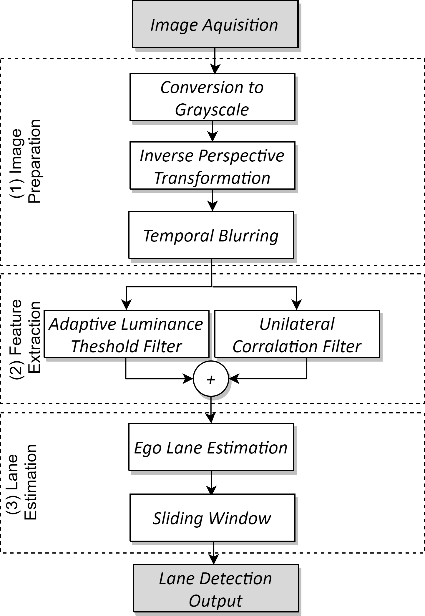
The first step is responsible for treating the image to obtain a better representation of the road. Initially, the image is reduced to a monochromatic color space scale, resulting in a single-channel one where each pixel is represented by 8 bits. Then, an IPM (Inverse Perspective Mapping) obtains a region of interest that mitigates noise and distortions, providing an aerial panoramic image of the road, or simply BEV image (Bird’s Eye View) (Li et al., 2019). Thus, we obtain in this step a grayscale image from an aerial perspective where the traffic lanes tend to be parallel and of constant width. A temporal integration technique is then used on the frames, increasing the quality of degraded lanes and further removing more unwanted information (Son et al., 2019). This last technique relies on the fact that markings do not vary considerably
in subsequent frames.
In the second step, we use two methods to highlight lane markings on the road and to reduce noise and unwanted information. Given the color variation of lanes, the algorithm uses a threshold adaptive filter based on the image luminance (Wu et al., 2019). It uses the brightness difference between the lane marks and the road to remove unnecessary information. Additionally, it uses a simple edge detector to obtain the vertical markings of the lanes (Zhang & Ma, 2019). Then, both feature maps are combined to obtain a version of the image that contains only the stripes’ markings.
The last step estimates the lane position by identifying its guiding straps and has two phases, as shown in Figure 1. Initially, a rectangular region at the lower portion of the image is set based on a pixel intensity histogram, so the region has the highest probability of including the lane’s traffic stripes. From this point, the system slides the window upward and laterally repositions the window to maximize the likelihood of finding the stripes (Cao et al., 2019). In this process, the window runs vertically over the image, estimating the position of the lane markings. The sliding window method obtains two sets of markings representing the lane in the BEV image.
Works related to the implemented algorithm
Images captured by cameras are usually in color, and many lane detection methods convert the images to grayscale (Huang et al., 2018; Li et al., 2019; Zhang & Ma, 2019) to simplify the problem. In addition, predefined regions of interest are used to remove external noise and reduce the amount of information processed.
In Lee and Moon , a detection algorithm was proposed based on using two regions of interest, a rectangular and a \(\Lambda\) shaped one. Wang et al., 2004 divides the region of interest into finite sections to make the traffic lanes tracking simpler, while Li et al. (2014) makes use of estimators to get straight segments from these regions. It is also possible to determine the region of interest using transforms to remove perspective distortions.
Some works use the inverse perspective mapping (IPM) to obtain an aerial panoramic image of the road (Bird’s Eye View, BEV) seeking an image where the traffic lanes tend to be parallel and of constant width (Borkar et al., 2012; Li et al., 2019; Raja Muthalagu et al., 2020).
Furthermore, the temporal blurring technique was proposed by Borkar et al., (2009) and Son et al., 2019 to improve the quality of degraded and worn traffic stripes. These methods perform a temporal integration of the previous frames to enhance the markings, increasing detection confidence.
The feature extraction method is employed in many works related to the subject (Borkar et al., 2012; Lee & Moon, 2018; Li et al. 2014; Jongin Son et al., 2015; Wang et al., 2004). In such algorithms, image processing seeks to detect the gradients, color patterns, and other information in the image’s pixels to recognize the traffic stripes. Additionally, seeking greater robustness to luminosity variations, Wu et al., 2019 proposes an adaptive luminance threshold filter to highlight the lanes and filter noise.
Lastly, a few works highlight the efficiency of the sliding window method for detecting the traffic lanes (Cao et al., 2019; Raja Muthalagu et al., 2020; Reichenbach et al., 2018). This technique combines a good detection rate accuracy and reduced computational complexity, viable to embedded real-time algorithms. In addition, the method can estimate the curvature of the road lane. For instance, in text citation
(Reichenbach et al., 2018), several methods for lane detection in embedded systems are evaluated.
Finally, some authors have addressed the lane detection topic considering the real-time constraints (Abdelhamid Mammeri et al., 2016; VanQuang Nguyen et al., 2018; Küçükmanisa et al., 2019; Selim et al., 2022), as discussed in the introduction. However, the literature has yet to address heterogeneous computing to improve the computational performance in the matter. Nevertheless, the works of Afif et al., 2020, Li et al., 2020, Jaiswal and Kumar 2020, and Zhi et al., 2019 discuss the benefits of CUDA-based algorithms benefits in other applications with image processing and real-time requirements, which may provide a background in the CUDA optimization techniques.
Acceleration of algorithms using CUDA
Architecture of a CUDA-based GPU
Unlike a traditional Central Process Unit (CPU), a Graphics Processing Unit (GPU) has an architecture that can effectively accelerate image processing and computer vision algorithms (Li et al., 2020). CUDA is a programming interface developed by NVIDIA to facilitate software development on GPU, and which has found wide use in the acceleration of image processing algorithms.
A modern GPU has Stream Multiprocessors (SM), which are independent units of decoding, instruction fetch, and execution (Sanders & Kandrot, 2010; Yonglong et al., 2013). SM are composed of dependent units, called Streaming Processors (SP), which are the basic units for thread execution on GPUs. These units are commonly called CUDA cores on NVIDIA chips.
The Maxwell architecture (Nvidia, 2014) features an enhanced SM. It is partitioned into four distinct processing blocks of 32 CUDA cores each (128 CUDA cores per SM). Each block has its features for instruction scheduling and buffering. This configuration provides a warp size alignment, making it easier to use and improving efficiency.
Shared memory allows threads from the same block to act cooperatively, facilitating the reuse of resources and mitigating transfers between slower off-chip memories (Nvidia, 2011; Yonglong et al., 2013). Heterogeneous programming using CUDA is split between host and device code. Each thread that runs on the device has a unique identifier, called threadIdx. A set of thread blocks form a thread grid. A kernel can run simultaneously in all threads of a grid. Each thread has its local private memory, while each block has a shared memory. All threads within that block can access the shared memory. Also, threads in a block have the same lifecycle as the block (Nvidia, 2011).
An NVIDIA Jetson Nano board is used to evaluate all the algorithms and to validate the method using a GPU architecture. The Jetson Nano is a commercial single board embedded computer composed by a quad-core ARM Cortex A57 CPU and an NVIDIA 128 core (1 SM) Maxwell architecture GPU. To run the method in real-time in such an embedded system, the algorithm must perform using the maximum GPU resources as possible. Thus, several CUDA optimizations were made to improve
efficiency.
The remainder of this section will discuss the usual optimizations applied to kernels (functions that are executed \(n\) times in parallel by \(n\) CUDA threads) that are part of the proposed method. The goal is to identify and mitigate the implementation bottlenecks. The following sections present detailed and specific CUDA optimizations. They classify into three types of implementation
bottlenecks:
memory bandwidth;
instruction latency;
instruction throughput.
The NVIDIA Visual Profiler, an NVIDIA profiling tool used to optimize CUDA applications, is used to help analyze kernel execution metrics, providing important feedback for optimization.
Memory optimization
In general, these optimizations seek to increase the memory throughput. They aim to minimize global memory accesses while employing the most suitable access pattern to realize memory coalescing, thus minimizing memory transactions.
One of the techniques is the use of shared memory for redundant and non-coalescing accesses. Shared memory is usually faster than global memory, i.e. has lower latency and higher bandwidth. The use of shared memory is especially profitable for unaligned data accesses.
It is also important to use the best access pattern according to each situation, ensuring coalesced access to global memory. Also, some optimizations were required, such as data transposition from an array of structures (AoS) to a structure of arrays (SoA), the use of padding, and changes to the parallelization strategy.
Latency optimization
Latency optimization aims to guarantee that there are as many threads as possible in execution to mask the latency effect. The block sizes must always be a multiple of the warp size to ensure that an entire warp performs the same operation, achieving higher occupancy and latency hiding. Grid size selection is crucial and was done empirically by comparing the performance of different sizes using the profiler.
Additionally, grid-strided loops are used for latency hiding. It provides an efficient solution to avoid monolithic kernels and ensure a higher occupancy.
Instruction optimization
Some kernels are compute-intensive, which can cause a bottleneck in instruction execution. Therefore, organizing and optimizing their operations is necessary to avoid that. The main objective of this type of optimization is to reduce the number of total instructions required to carry out an operation. One of the techniques adopted is using high-throughput operations, such as SIMD (Single Instruction, Multiple Data) and SIMT (Single Instruction, Multiple Threads) warp-level primitives.
Those are instructions that perform operations with larger data blocks. Several operations were vectorized in a grid-strided loop using the data arrangement to ensure the highest execution efficiency. Also, we seek to avoid branch divergence in warps and reduce bank conflicts.
Image preparation and inverse perspective mapping
There are an unlimited amount of scenarios for driving a car. Naturally, there is plenty of content irrelevant to the problem in the captured image. Therefore, it is a common strategy to pre-process the input image followed by the feature extraction technique (Hillel et al., 2014; Sandipann P. Narote et al., 2018; Yenikaya et al., 2013). This processing step has been applied to images to reduce noise and external distortions, providing a better region of interest and reducing the amount of processed data. Doing so also increases the reliability of the input data (Sandipann P. Narote et al., 2018). This section details the pre-processing employed in our technique, which includes image preparation, IPM transformation, and temporal blurring.
Image preparation
Transforming the three-color channel RGB image to grayscale reduces its size to a third of the original and minimizes the brightness interference over the three-channel image. Furthermore, it simplifies the problem and algorithms when seeking embedded processing (Huang et al., 2018; Li et al., 2019; Sandipann P. Narote et al., 2018; Zhi et al., 2019).
Processing the grayscale conversion has a higher degree of parallelization. Given that all operators are simple, the throughput is limited only by the memory bandwidth. Patterns of 16 bytes are read in each loop and loaded to the shared memory to ensure better efficiency when accessing the main memory, where the access is strided without performance loss. These patterns are converted from an AoS to SoA, such as discussed in the Memory optimization section before. Furthermore, all operations are vectorized, increasing the number of pixels processed in each iteration. The conversion to gray in 16 pixels is computed through structures that allow isolated access to this information.
Inverse perspective mapping
In the lane detection problem, the camera typically faces forward and causes a perspective distortion. Such distortion shows the lane markings tending to a vanishing point, disobeying a few assumptions. The main problem is that the traffic lane stripes lose the characteristic of being parallel to each other, so the two markings that define a lane become close as they are away from the camera. The lane curvature estimation becomes more complex and less predictable (Yu & Jo, 2018).
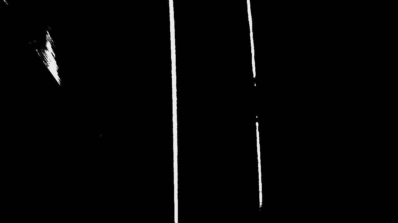
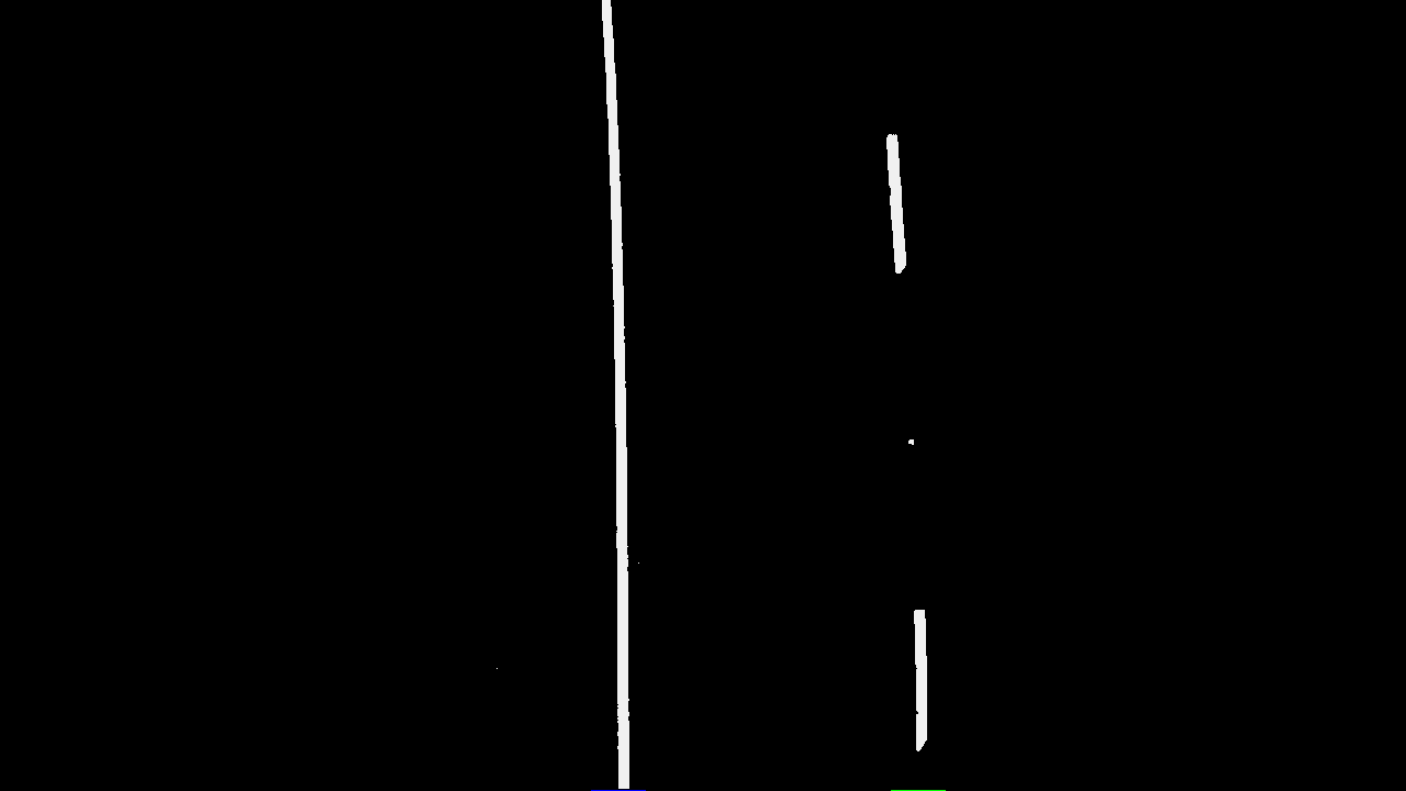
These assumptions are inherent characteristics of transit lanes, and computer vision algorithms can use these parameters to fine-tune their operation. To re-establish the characteristics of the road, several works (Li et al. 2014; Raja Muthalagu et al., 2020; Sivaraman & Trivedi, 2013) perform a change of perspective to obtain an aerial image (BEV) through the inverse perspective mapping (IPM). Figure 2 shows a diagram of the perspective change in this processing.
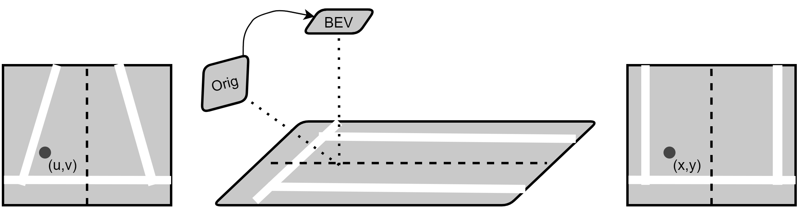
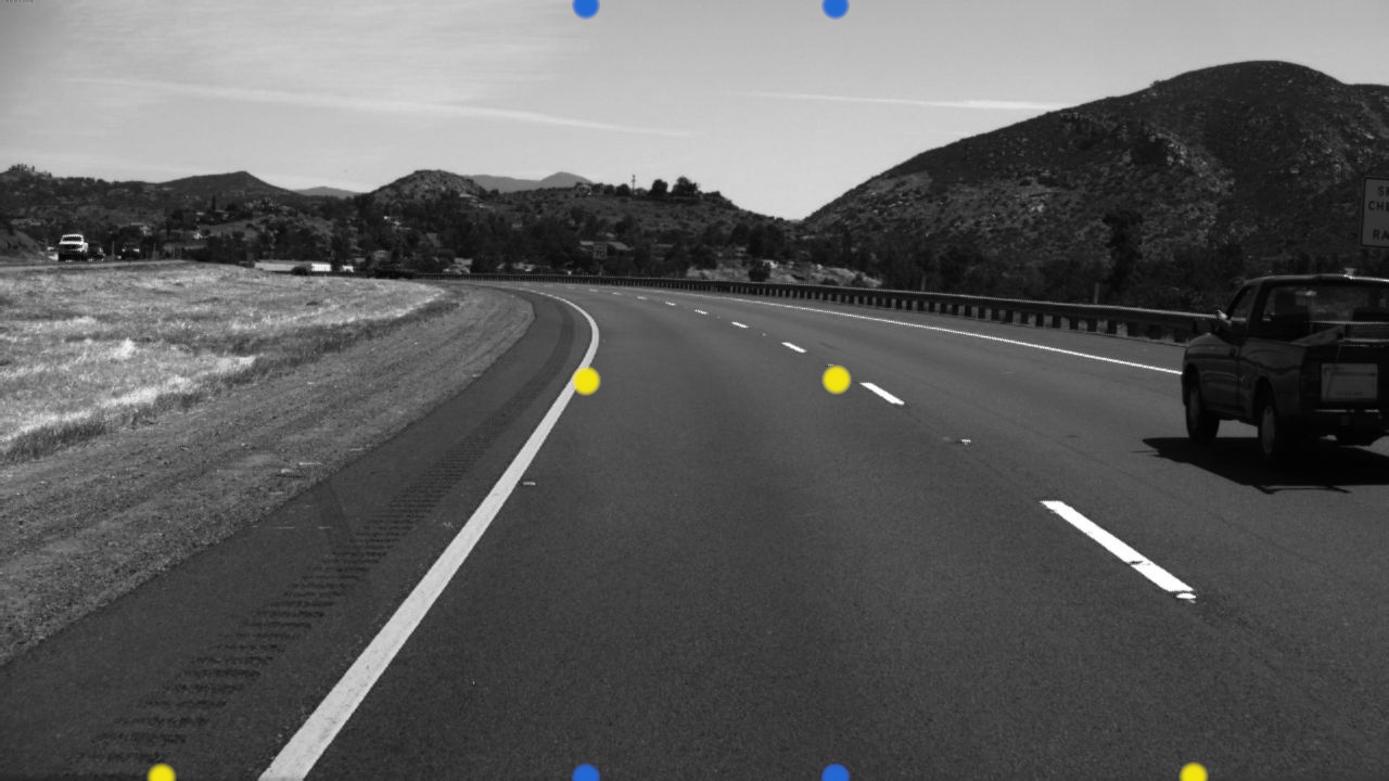
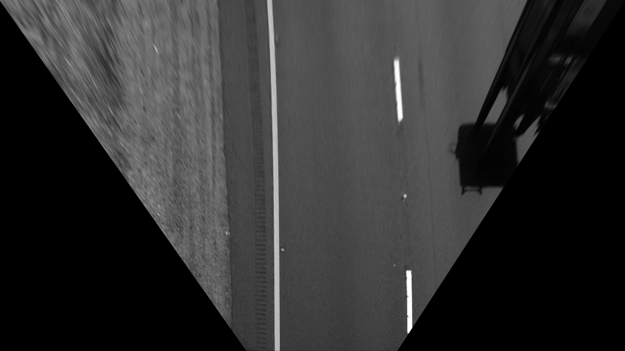
This operation is a projective transformation with eight degrees of freedom that can be constrained by several elements present in the image. The eight degrees of freedom are obtained by selecting 8 points on the image, which allows for solving the homography directly. Homography is the transformation relation between two planes formed by the corresponding 8 points, with 4 points in each plane (Hartley & Zisserman, 2003). Figure 3(a) shows an example of these points. This homography translates into a third-order matrix, responsible for transforming a point in the original image into a point in the BEV perspective image, as shown in Figure 3(b). There are two methods to obtain this matrix:
dynamically during execution (Paula & Jung, 2015);
using a pre-computed static manner (Huang et al., 2018; Raja Muthalagu et al., 2020).
The dynamic way has greater computational complexity and depends on a specific trigger sequence. The static method is more susceptible to variations but has a minimal computational cost, thus making it suitable for real-time embedded processing.
(a)
(b)
Using the homography matrix \(H\) it is possible to obtain the pixels of the transformed image \(I(x,y)\) as a function of the input image’s pixel \(O(x,y)\) through equation (1) (Huang et al., 2018; Raja Muthalagu et al., 2020)
(1)
\[ I(x, y)=O\left(\frac{H_{11}x + H_{12}y + H_{13}}{H_{31}x + H_{32}y + H_{33}}, \frac{H_{21}x + H_{22}y + H_{23}}{H_{31}x + H_{32}y + H_{33}}\right).\]
Equation (1) can produce float points coordinates that do not belong to the image. The workaround is to calculate the original image pixels (\(I\)) to each of the transformed ones (\(O\)). This approach provides an output image without interference, and it avoids the calculation of about 45% of the total pixels because of the transformation characteristics, e.g., the two black triangles in Figure 3(b). The operations were vectorized to ensure a higher throughput and thus improve performance. Besides, some terms in equation (1) are constant for a couple of pixels, which allows to keep those calculations in the registers and reuse them in other ones.
Temporal blurring
The temporal blurring improves the lane markings by making them more robust and obscuring moving objects, reducing possible sources of external noises. One of the expected effects is that lanes with discontinuous straps or worn ones will have a more uniform and continuous appearance (Borkar et al., 2009), providing better detection quality (Silva et al., 2020)
.
The technique exploits the assumption that lanes do not change abruptly in a short period (in this case, in subsequent frames), especially when compared to other road objects (vehicles, pedestrians, etc.). Thus, an amount of \(N\) previous frames are temporally integrated to increase the confidence of the markings. By combining these images, the marks are overlapped, increasing the amount of information in the lanes. An example of the temporal blurring effect is shown in Figure 4.
(a)
(b)

The temporal frame integration (Son et al., 2019) is performed by means of equation (2)
(2)
\[ I_{avg} = \sum^{N}_{i=0} \frac{I(n-i)}{N},\] where \(I_{avg}\) is the resulting image with \(N\) previous frames combined.
Unlike previous kernels, the data is already allocated within the GPU memory, and given that it performs simple operations, the bandwidth is the major limitation. The reading bandwidth is maximized using a grid-stride loop to ensure a higher occupancy, minimizing latency.
Feature extraction
The feature extraction procedure seeks to obtain an image with highlighted markings features and mitigating further useless information for the detection method. The method assembles feature maps that filter different characteristics of the marking. The maps are then combined to obtain a better result.
Adaptive threshold feature map
The lane markings tend to be the elements with the highest brightness in the image or, at least, brighter than the lanes themselves. Therefore, the first feature map highlights the markings based on the difference between pixel values and the average luminance. Fixed thresholds filters are inadequate due to ambient variation, such as asphalt and marking colors. The solution is to use an adaptive threshold filter based on the average luminance of the region of interest (Son et al., 2019; Wu et al., 2019).
The adaptive threshold calculates an average of the intensity (\(L_{avg}\)) of each pixel to the given region of interest. Based on that value, it estimates a inferior (\(T_L\)) and superior (\(T_U\)) threshold, as shown in equation (3):
(3)
\[ T_{L},~ T_{U} = \left\{ \begin{array}{cl} ~60 ,~ 220 & \text{if} \ 0 ~~\leq L_{avg} \leq 25, \\ 115 ,~ 235 & \text{if} \ 25 < L_{avg} \leq 40, \\ 125 ,~ 240 & \text{if} \ 40 < L_{avg} \leq 70, \\ 135 ,~ 250 & \text{if} \ 70 < L_{avg} \leq 100,\\ 145 ,~ 255 & \text{otherwise}. \end{array} \right.\]
Subsequently, each pixel of the image is then binarized using equation (4):
(4)
\[ I(x, y) = \left\{ \begin{array}{cl} 1 & \text{if} \ T_{L} \leq I(x,y) \leq T_{U},\\ 0 & \text{otherwise}. \end{array} \right.\]
Figure 5(b) presents an example of this feature map, where white traces represent the possible traffic lane markings.
(a)
(b)
To implement this procedure there are two kernels. The first calculates the average pixel intensity of the image, while the second performs the binarization using equation (4) and the threshold values.
Considering the image already allocated within the GPU memory, the kernel uses a grid-stride loop to maximize the reading bandwidth. Furthermore, batches of 128 bits are read and then written at the shared memory. The calculation of the sum of the pixels is vectorized to compute 16 pixels simultaneously.
The grid-stride loop is done by summing all input bytes of the data. After the operation, the threads from this block are reduced to a single value. This is done using the SIMT operator (__shfl_down_sync) available at the CUDA (synchronous reduction to each GPUs warp). At last, we make the atomic sum of the accumulated values at each warp, obtaining the total sum of the pixels.
The second kernel is responsible for making the image binarization using \(T_L\) and \(T_U\) values. It has a low computational cost as previous kernels that are bandwidth bound. To increase the throughput, it uses a set of SIMD instructions. Those are logical operators like setting if greater than (__vsetgtu4), setting if lower than (__vsetltu4), and unsigned minimum (__vminu4). The operators run in groups of 4 bytes each per iteration of the grid-stride loop.
Unilateral correlation feature map
Conventional edge detectors are unsuitable for real-time embedded system implementation due to their computational cost. This work uses a unilateral correlation filter (Zeng et al., 2015; Zhang & Ma, 2019), as the solution. This type of filter has a lower computational complexity and it is based on the convolution of the image with a separable convolution kernel.
The implemented filter is a third-order matrix that extracts a single type of edge in the image. As lane markings are almost vertical in the BEV image, the filter is designed to extract vertical edges, detecting horizontal variation of pixels.
Figure 6 presents an example of the feature map obtained by processing the unilateral correlation filter.
(a)
(b)
The filter also has the property of being separable. Therefore, it is possible to replace the \(3\times3\) convolution of the filter by two convolutions using the vectors \(\left[1 , 2, 1\right]\) and \(\left[-1, 0, 1\right]\). This property decreases the computational cost of the operation from \(O\left(m\times n\right)\) to \(O\left(m+n\right)\).
The kernel implemented for this part uses several optimizations aforementioned, such as the grid-stride loop, shared memory allocation, and operation vectorization. However, its implementation uses the tilling pattern, which are two-dimensional structures of threads (Kirk & Hwu, 2016), exploiting the intrinsic characteristics of the operation. This kernel uses sub-matrices to carry large amounts of information from the main to the shared memory, allowing strided access for calculation. Furthermore, due to the filter’s features, some of the values can be pre-computed and reused in other operations, reducing the number of operations performed in each loop.
Lane detection
The lane detection step has two stages. First, it detects regions most likely to contain the markings, and then, it estimates the points belonging to each of the markings. The first uses a column histogram algorithm to obtain the regions with the highest pixel density. The second uses these regions to initiate an iterative sliding window method that detects the pixels belonging to the
lane markings.
Column histogram
The column histogram operation determines the regions with the highest probability of containing the traffic lanes based on the intensity of the pixels in each column (Cao et al., 2019; Reichenbach et al., 2018). This is achieved by accumulating the value of each column of the feature map in Figure 7(a). The peaks obtained in this histogram are considered as candidates, such as the example of Figure 7(b).
(a)
(b)

This kernel responsible for the column histogram is one of the most complex, thus it has a higher degree of parallelization and can greatly benefit from the optimizations. It is possible to use the shared memory to ensure efficiency in memory access, grid-strided loops, and also instructions optimizations.
The kernel operation adopts a two-dimensional block to launch the threads. The shared memory stores the input data and allocates the positions and values used across the process. Operations were parallelized to improve the throughput and warp-level primitives are employed. Furthermore, the operation is symmetric and so it is possible to launch two similar blocks. Each one is responsible for processing one side of the image, making use of the problem’s geometry to ensure greater efficiency.
Another important aspect is that the kernel obtains only the initial position of the markings. Therefore, only the inferior half of the image is analyzed.
The warp-level primitive __shfl_down_sync is used twice to obtain the maximum value in each block. The first time it seeks the peaks of each warp. Then we use it again to get the global peaks. The first block obtains the peak referring to the left side of the image (left lane marking), while the second block obtains the one on the right.
Sliding windows
To detect the lane stripes’ positions, we group the regions with a higher density of pixels on the feature maps. The typical approach to obtain these positions is to process the entire image storing them. The issue with embedded execution is that such an approach is inefficient, as only a minor portion of the pixels contain lane markings information. This search can be optimized using the sliding windows method (Cao et al., 2019; Raja Muthalagu et al., 2020; Reichenbach et al., 2018), which evaluates only the regions of the image that are more likely to contain the lane marks.
Based on the points estimated by the column histogram algorithm, this technique places windows at those positions and then runs vertically over that region. Each window computes the peak of its respective small area. At the end of the process, each peak describes a point of the lane. Figure 8 shows an example of the procedure. The windows at the bottom depict the starting points, and then it vertically has the remainder of the windows. The blue circles per window represent the points with the highest probability of composing the lane.
(a)

(b)
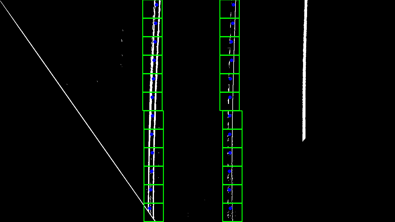
Instead of performing over the entire image, the operation is performed only on two regions using the geometry of the lanes. To improve the performance, we launch a tri-dimension grid of threads exploring the inherent parallelism of the operation. The x and y-axis are the sizes of the windows, and the z-axis is the other windows on that same lane.
The global memory data is loaded into the shared memory to ensure strided access. A column histogram computes the peak for each window using warp-level primitives, similarly to the previous kernel. To improve this operation the size of the windows should fit an integer number of warps.
Simulation test experiment
Results are divided into qualitative and quantitative analysis, as well as the execution time performance. The first subsection briefly discusses the setup and the dataset used during the tests, followed by the results and, at last, by a discussion and comparison with other works.
Test Environment and the Tusimple dataset
The test environment uses the NVIDIA Jetson Nano board and its GPU, discussed previously. For reference, the algorithms were developed in C++ language version 7.5.0 and the heterogeneous implementations were programmed using the CUDA 10.2 API.
The experiment uses images available in the TuSimple dataset. It has three subsets totaling 3626 video clips (72520 frames) with roads comprising annotated image frames of US highways. Each image has a 1280x720 resolution captured by a camera in the middle of the vehicle’s windshield. The dataset consists of small scenes made of a varying number of 1-second clips. Each of these clips contains 20 frames, and the last one has an annotation of the polyline types for lane markings. Each scenario may have different weather conditions at various times of the day. Furthermore, they are taken on different types of roads and under arbitrary traffic conditions.
Apart from the theoretical discussion before, there are two characteristics of the algorithms calibrated and tailored based on the TuSimple datasets’ images.
These are the homography matrix \(H\) and the sliding window format. The former is calibrated offline based on the camera’s output image (Silva, 2021b), and the region of interest obtained by the IPM transformation uses the matrix \(H\) given in equation (5):
(5)
\[ H = \left[ {\begin{array}{*{20}{c}} { - 0.05}&{ - 2.8630}&{1002}\\ 0&{ - 4.0855}&{1429}\\ 0&{ - 0.0043}&1 \end{array}} \right].\]
The latter was set to a size of \(32\times30\) pixels, which is identical in numbers to the number of threads (32 horizontals and 30 verticals) deployed in the CUDA algorithm, optimizing the operation. In addition, the temporal blurring integrates 20 frames (\(N=20\)), such as the example in Figure 4(b). The remainder of the steps follows the characteristics discussed before.
Qualitative analysis of ego-lane detection
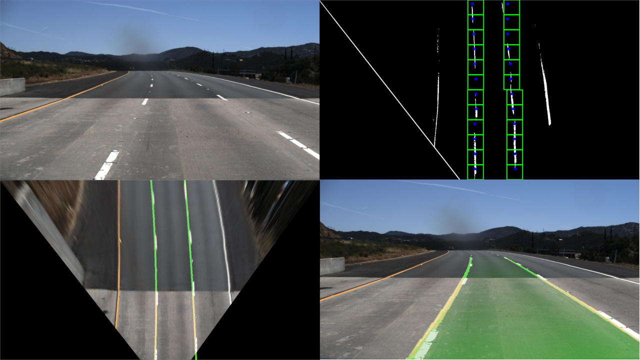
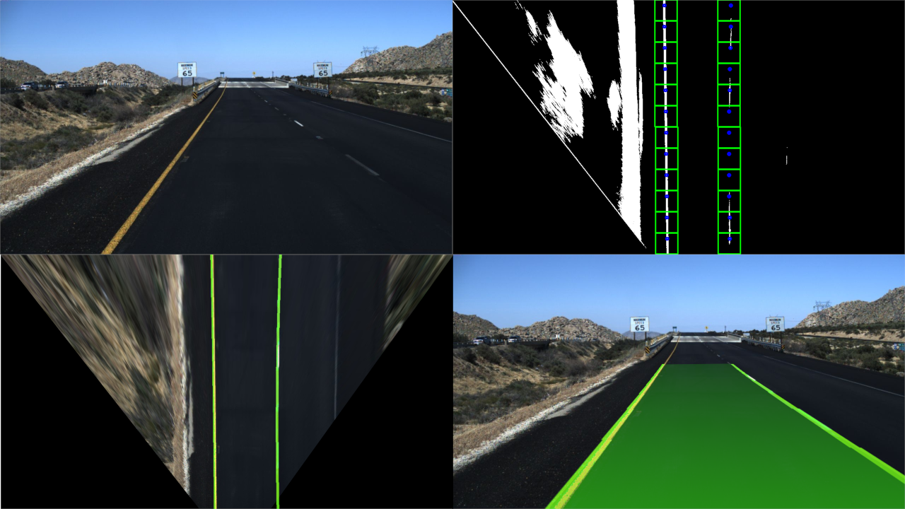
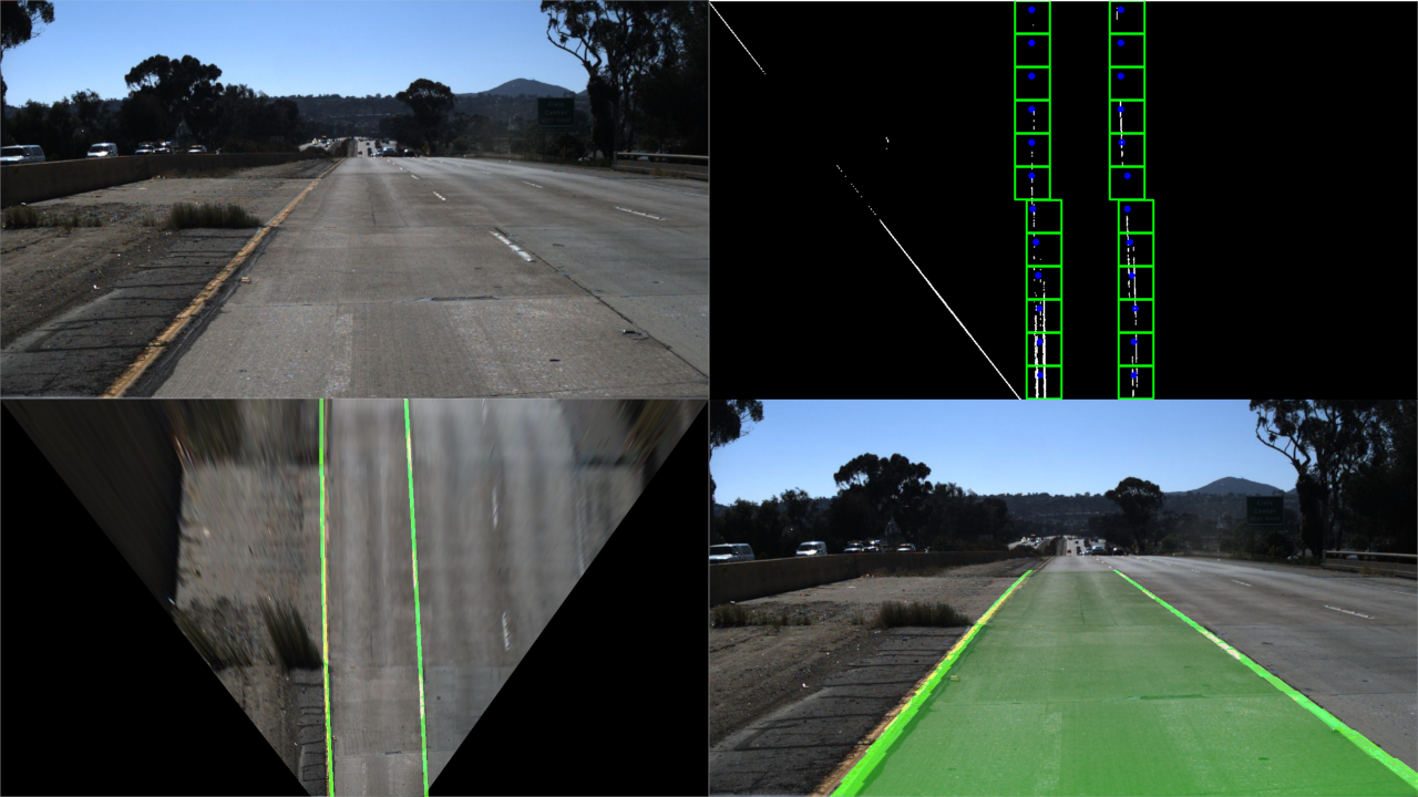
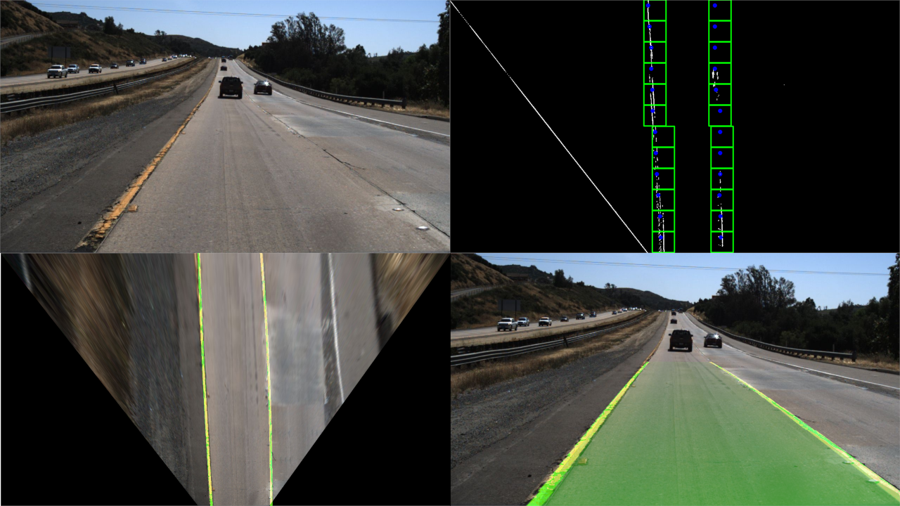
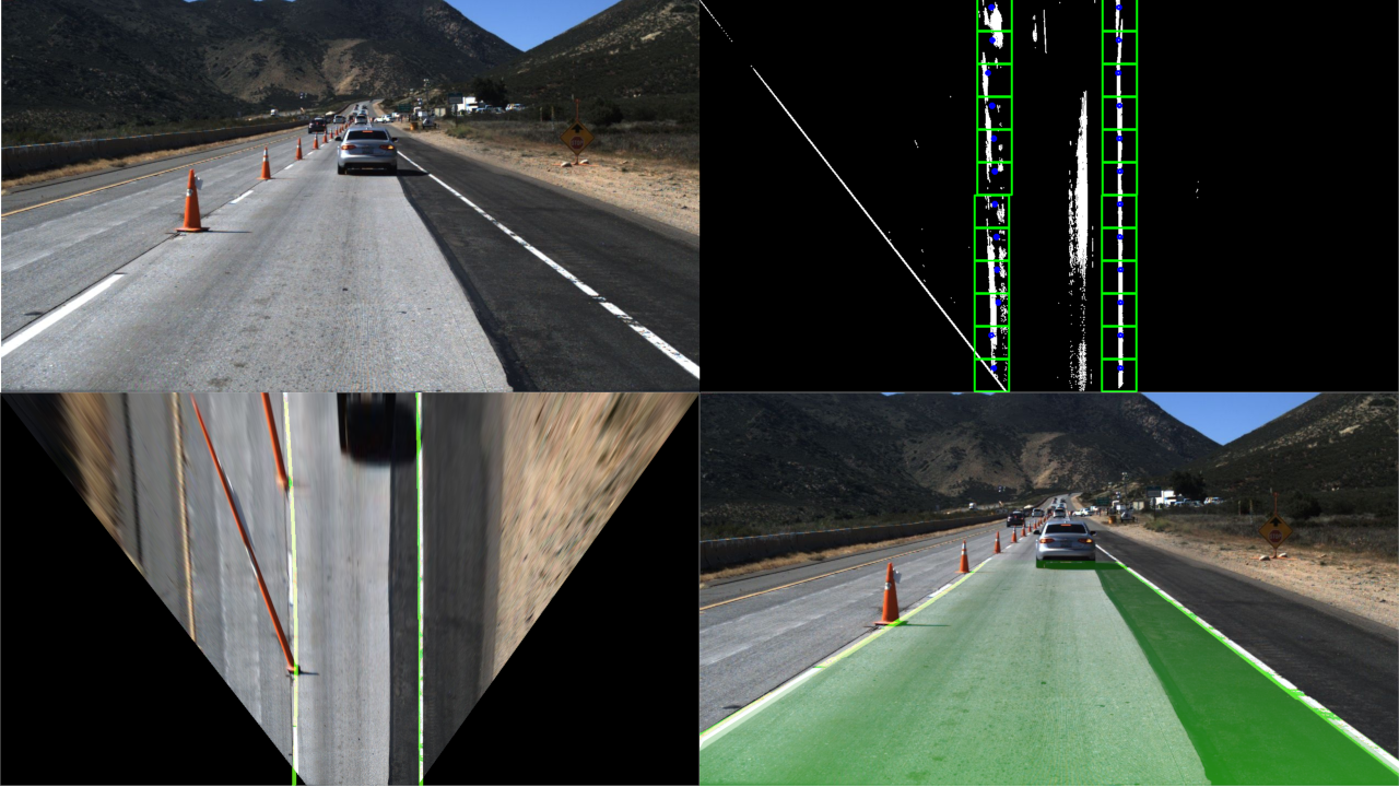
We use different scenes from the dataset to analyze the algorithm’s parts response comparing it for different implementations. Figures 9(a)-(f), shows some examples. Each element in Figure 9 consists of four images showing: the original figure (upper left corner), the sliding window output (upper right corner), the adjustment of detected ranges in the BEV perspective (lower left corner), and the final output (lower right corner). Those six scenes exemplify the algorithm’s response in different cases and types of roads to the reader.
| (a) |
 |
| (b) |
 |
| (c) |
 |
| (d) |
 |
| (e) |
 |
| (f) |
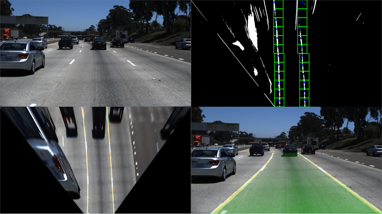 |
Figures 9(a) and 9(b) show results from roads with distinct asphalt colors and internal coloring variations. Figure 9(c) is an example of a very dark asphalt with worn lane markings. Even in this scenario, the feature extraction performance is satisfactory, and the algorithm performance is maintained. Other cases with degraded asphalts and worn markings are shown in Figures 9(d) and 9(e), where the image preparation and the BEV perspective are fundamental for improving the
detection.
The perspective transformation also reduces the complexity of lane detection with curvatures. Figures 9(a) and 9(f) are examples of that. Those results show the algorithm has satisfactory ego-lane detection even under the least favorable circumstances, including worn asphalts and markings, curvatures, and color variations.
The video in Silva (2021a) illustrates the operation of our algorithm. The video shows the images available on the Tusimple dataset 0601. That dataset comprises a sequence of 8200 frames assembled as a motion picture of 1-second clips. We split the image into quadrants: The upper left corner shows the original video. The upper right shows the preprocessed video by the method.
The lower left shows the resulting feature map with the windows (formed by the green rectangles) and the detected dots in blue. The last shows the original video with its frames overlapped by dots marking the estimated road stripes.
Algorithm performance
Table 1 shows the proposed method’s operations execution times for three distinct solutions. The first column presents the execution times for the optimized heterogeneous algorithm using CUDA. The second brings the times for an intermediate implementation, which uses the graphic chip through the OpenCV library and CUDA. The last shows the execution times for the embedded system’s CPU implementation. The values obtained in each function do not consider the loading and storing times of the image.
| Operation | CUDA | OpenCV | CPU |
|---|---|---|---|
| Conv. grayscale | 0.269 | 1.320 | 48.514 |
| IPM | 0.305 | 20.913 | 97.181 |
| Temporal blurring | 0.763 | 2.834 | 33.346 |
| Adapt. threshold | 0.139 | 0.917 | 42.109 |
| Uni. correlation | 0.677 | 19.564 | 62.887 |
| Column Histogram | 0.081 | 7.091 | 38.348 |
| Sliding Windows | 0.106 | 8.603 | 9.098 |
| Total runtime | 2.34 | 61.242 | 331.483 |
Table 2 summarizes the speed-ups of the proposed method in comparison with the other two.
| Operation | CUDA \(\times\) CPU | CUDA \(\times\) OpenCV |
|---|---|---|
| Conv. Grayscale | 180.3 | 4.9 |
| IPM | 318.6 | 68.5 |
| Temporal blurring | 43.7 | 3.7 |
| Adapt.s threshold | 302.9 | 6.6 |
| Uni. correlation | 92.9 | 28.9 |
| Column Histogram | 473.4 | 87.5 |
| Sliding Windows | 85.8 | 81.1 |
| Total speed-up | 141.6 | 26.1 |
The results show that the runtime of the heterogeneous implementation is significantly better than the others. The optimized algorithm is 25 and 140 times faster than the intermediate and the CPU methods, respectively. Naturally, the execution time gain varies depending on the algorithm’s part. At specific components, it is possible to observe that the proposed implementation achieves much higher performance, even compared to the version running on the GPU compiled in OpenCV.
In the CPU-based approach, processing a single frame took over 300 milliseconds, equivalent to approximately three frames per second (fps). The runtimes obtained demonstrate the inability to meet the criteria for a real-time application. The main reason for this long time is the image processing operations, which are serialized. A typical camera (or video) has 30 fps, and the time between frames is reasonable to assume as the minimum for a real-time application.
The OpenCV approach had a speed-up of approximately 5.5 times compared to the CPU one, processing a single frame every 60 milliseconds or 16 fps. Much of the improvement is due to the speed-up of image processing operations, such as conversion to grayscale, adaptive threshold, and temporal integration. Despite a significant improvement, the implementation still does not meet the necessary criteria for real-time execution.
Finally, the proposed heterogeneous method can process a frame in less than three milliseconds. That is equivalent to processing over 300 fps and complying with a real-time requirement. It is evident that to maximize the performance on the GPU, the parallelization of the methods is necessary. It is worth noting that since the algorithm runs at least five times faster than the minimum required for a real-time application, it would still be possible to implement other features in the lane detection method. Additional implementations in the algorithm could further improve the detection quality without preventing the real-time requirement.
Quantitative analysis of ego-lane detection on Tusimple dataset
The benchmark compares the ego-lanes obtained by the algorithm with the ground truth. Thus, we demonstrate that the method using heterogeneous computing is capable of detecting the lane markings accordingly and is suitable for embedded applications.
It is possible to evaluate the quality of the lane markings estimation using the ground truth available in each clip of the dataset comparing with the results obtained by the proposed algorithm. The principal quality metric evaluated is the accuracy (ACC), described
by
(6)
\[ \text{ACC} = \frac{\sum_{clip} P_{valid}}{\sum_{clip} P_{total}},\] where \(P_{valid}\) corresponds to the number of correct points and \(P_{total}\) to the number of total points.
Equation (6), measures the rate of valid estimates made by the method compared to the ground truth. An estimated point is valid if the difference between the true and estimated point is less than a threshold
value (\(T_{pixel}\)).
In addition to validating each point in the lane, it is necessary to validate the lane itself. A detected lane is said to be valid if it has at least \(T_{point}\)% of valid points, as shown in equation (7):
(7)
\[ \text{Matched}= \frac{M_{pred}}{N_{pred}},\] where \(M_{pred}\) is the number of matched predicted lanes, \(N_{pred}\) is the number of all predicted lanes. Similarly, equation (8) measures the rate of markings estimated by the method that does not match the ground truth ones:
(8)
\[ \text{FP} = \frac{F_{pred}}{N_{pred}},\] where \(F_{pred}\) is the number of wrong predicted lanes. \(\text{Matched}\) represents the lane rate and FP the false positive rate.
The results of \(\text{ACC}\), \(\text{Matched}\) and \(\text{FP}\) obtained for the TuSimple dataset are arranged in Table 3. The data presents values for a \(T_{pixel}\) of \(20\) px, \(35\) px, and \(50\) px, and \(T_{points} = 80\)%.
| Dataset | T\(_{\text{Pixel} }\) (px) | ACC (%) | Matched (%) | FP (%) |
| 0313 | 20 | 81.3 | 74.0 | 26.0 |
| 35 | 88.4 | 84.4 | 15.6 | |
| 50 | 92.2 | 87.7 | 12.3 | |
| 0531 | 20 | 90.0 | 87.7 | 12.3 |
| 35 | 95.2 | 94.8 | 5.2 | |
| 50 | 97.3 | 95.9 | 4.0 | |
| 0601 | 20 | 92.3 | 91.0 | 9.0 |
| 35 | 97.2 | 97.3 | 2.7 | |
| 50 | 99.0 | 97.9 | 2.1 |
The ACC rate of the proposed method ranged from \(81.3\)% to \(99.0\)%, in the worst and best performance, respectively. The dataset 0313 detection rate is degraded because most images are taken from roads with non-reflective raised pavement markers called Botts’ dots in place of painted lane marks. These Botts’ dots are usually yellow or white. White-colored dots on concrete pavements will turn a pavement-like color due to dirt. The feature extraction algorithm is optimized for traditional traffic stripes and not such markings. On the other hand, dataset 0601 has long stretches of lanes with signaling in good condition, ensuring better results.
The proposed method performed well under the different conditions present in the datasets. The results were satisfactory even for the unconventional lanes present in dataset 0313. The overall average accuracy values for the different \(T_{pixel}=20\) px, \(35\) px, and \(50\) px are respectively \(91.2\)%, \(96.2\)%, and \(98.1\)% when disregarding such markings. Comparison with other works and algorithms, both in terms of accuracy and computational complexity, is presented next.
Comparison with other methods and discussions
Table 4 places the proposed method in the lane detection scenario. It concisely presents the performance of other works, including similar methods for ego-lane and multi-lane detection. All values are from their respective publications. Thus, we can make a reasonably fair comparison between the methods. But we must consider that they run on different systems, where some use other datasets and apply different methodologies to establish their metrics. However, the comparison shows strong evidence that the proposed method performs better considering embedded real-time applications.
| Method | Algorithm | Average Detection | Avg. Proces. Time (ms) per Frame | Input Resolution | System Environment |
| Multi-lane | (Son et al., 2019) | 98.9 | 667.0 | 640x360 | Intel Core i7-4th |
| Ego-lane | (Wu et al., 2019) | 96.33 | 261.1 | 1280x720 | Intel Core i7-2th |
| Multi-lane | (Zheng et al., 2018) | 95.7 | 65.4 | 768x432 | Intel Core i7-6th |
| Multi-lane (deep leaning) | (Philion, 2019) | 97.25 | 65.3 | 1280x720 | NVIDIA GTX 1080, GPU |
| Ego-lane | (Raja Muthalagu et al., 2020) | 95.75 | 63.6 | 1280x720 | Intel Core i5-6th |
| Ego-lane | (Kühnl et al. 2012) | 94.40 | 45.0 | 800x600 | NVIDIA GTX 580 GPU |
| Multi-lane (deep learning) | (Zou et al., 2020) | 97.25 | 42.0 | 1280x720 | Intel Xeon E5-2th GTX TITAN-X GPU |
| Multi-lane (straight) | (Kim et al. 2016) | 98.10 | 34.0 | 640x480 | NVIDIA Jetson TK1 board |
| Multi-lane | (Cao et al., 2019) | 98.42 | 22.2 | 1280x720 | Intel Core i5-6th |
| Ego-lane | Proposed Solution | 98.15\(^{*}\) | 2.34 | 1280x720 | NVIDIA Jetson Nano board |
| 96.15\(^{**}\) |
\(^{*}\)Results without the TuSimple dataset 0313.
\(^{**}\)Results with the TuSimple dataset 0313.
The deep learning methods (Philion, 2019; Zou et al., 2020) perform multi-lane detection using the TuSimple dataset. They show high detection rates and approach real-time execution, even performing a more complex task than ego-lane detection. However, both works report running their methods on desktops with dedicated graphics processing systems. Therefore, they have far superior processing capabilities than a GPU integrated into an embedded system, which would extrapolate the limited resources of the latter.
The works of Kühnl et al. (2012), Wu et al., 2019 and Raja Muthalagu et al., 2020 present solutions for ego-lane detection using conventional desktop computers. Their detection rates are slightly lower than the other methods that also use desktops. Among them, the fastest one utilizes lower-resolution images and a dedicated GPU card.
The authors in Kim et al. (2016) present an even simpler multi-lane detection solution, which approximates the lanes to straight lines, not detecting the curvatures. It features a high detection rate but uses a low-resolution image, directly impacting the runtime and quality of these detections. However, unlike the other proposed methods, it achieves requirements close to real-time in an embedded system.
From the average processing time per frame in Table 4, only the proposed method can satisfy the real-time criteria established in this work. The optimization performed by the heterogeneous implementation using CUDA leads to an average processing time of 2.34 ms. That indicates the proposed method is executed using only part of the processing power and capabilities of a GPU tailored for embedded systems. Additionally, its average detection rate, excluding the TuSimple subset 0313, was approximately 98%. These results demonstrate the feasibility of implementing our method in embedded systems. Furthermore, adding improvements or new features to the algorithm is possible without compromising the real-time criteria.
Conclusions
This work presents a viable solution for ego-lane detection using a low-cost embedded platform. The proposed solution using heterogeneous computing based on CUDA shows that performance can be boosted significantly compared to non-optimized solutions, such as OpenCV implementations.
The method performs within the established real-time limits. The embedded system processes each frame in approximately 2.34 ms, 25 times faster than the OpenCV GPU-compiled version and 140 times faster than the CPU-executed sequential version. Additionally, considering the method’s run-time, which is superior to 400 frames per second, future implementations can improve even further and enhance the detection quality, still coping with the real-time criteria. Hence, other state-of-the-art algorithms can be implemented and optimized similarly to those reported, or the same GPU could execute other tasks besides the ego-lane detection algorithm.
Moreover, the algorithm proved efficient for detecting ego-lane on roads and highways running TuSimple dataset images with different scenarios. The method’s performance ranged from 92.3% to 99.0% accuracy in the best subset, detecting up to 97.9% of the ego-lane available with 80% of the valid points. In this way, the work is in the same range as other similar methods, with the difference of being executed in an inexpensive graphics-processing-tailored real-time embedded system.
Future works may assess the CUDA implementation in other algorithms, such as deep learning, convolutional neural networks, pixel-level classification networks, and others. Hence, it would be possible to evaluate if these more computationally costly methods could perform in real-time in typical embedded systems while seeking to increase detection rates, especially in unconventional lane conditions such as those of the TuSimple 0313 dataset.
Author contributions
G.B. Silva participated in the: Conceptualization, Data Curation, Programs, Formal Analysis, Investigation, Methodology, Validation, Writing – original draft. D.L. Gazzoni Filho participated in the: Formal Analysis, Programs, Methodology, Investigation, Writing – Revision. D.S. Batista and M.C. Tosin participated in the: Methodo-logy, Visualization, Writing – Original Draft and Revision. L.F. Melo participated in the: Resources, Project Managements, Writing – Revision.
Conflicts of interest
The authors declare no conflict of interest.
Acknowledgments
This study was financed in part by the Coordenação de Aperfeiçoamento de Pessoal de Nível Superior – Brasil (CAPES) – Finance Code 001.
References
Yonglong, Z., Kuizhi, M., Xiang, J., & Peixiang, D. (2013). Parallelization and Optimization of SIFT on GPU Using CUDA. In Institute of Electrical and Electronics Engineers, Conferences [Proceedings]. 10th International Conference on High Performance Computing and Communications & 2013 IEEE International Conference on Embedded and Ubiquitous Computing. Zhangjiajie, China.
Sanders, J., & Kandrot,E.(2010). CUDA by Example: An Introduction to General-Purpose GPU Programming. Addison-Wesley Professional.
Afif, M., Said, Y., & Atri, M. (2020). Computer vision algorithms acceleration using graphic processors NVIDIA CUDA. Cluster Computing, 23(4), 3335–3347. https://doi.org/10.1007/s10586-020-03090-6
Cao, J., Song, S., Xiao, W., & Peng, Z.(2019).Lane detection algorithm for intelligent vehicles in complex road conditions and dynamic environments. Sensors, 19, 3166. https://doi.org/10.3390/s19143166
Hillel, A. B., Lerner, R., Levi, D., & Raz, G. (2014). Recent progress in road and lane detection: A survey. Machine Vision and Applications, 25, 727–745. https://doi.org/10.1007/s00138-011-0404-2
Kim, J., Kim, J., Jang, G.-J., & Lee, M. (2017). Fast learning method for convolutional neural networks using extreme learning machine and its application to lane detection. Neural Networks, 87, 109–121. https://doi.org/10.1016/j.neunet.2016.12.002
Lee, C., & Moon, J.-H. (2018). Robust Lane Detection and Tracking for Real-Time Applications. IEEE Transactions on Intelligent Transportation Systems, 19(12), 4043–4048. https://doi.org/10.1109/TITS.2018.2791572
Li, J., Deng, G., Zhang, W., Zhang, C., Wang, F., & Liu, Y. (2020). Realization of CUDA-based real-time multi-camera visual SLAM in embedded systems. Journal of Real-Time Image Processing, 17(3), 713–727. https://doi.org/10.1007/s11554-019-00924-4
Mammeri, A., Boukerche, A., & Tang, Z. (2016). A realtime lane marking localization, tracking and communication system. Computer Communications, 73, 132–143. https://doi.org/10.1016/j.comcom.2015.08.010
Muthalagu, R., Bolimera, A., & Kalaichelvi, V. (2020). Lane detection technique based on perspective transformation and histogram analysis for selfdriving cars. Computers & Electrical Engineering, 85, 106653. https://doi.org/10.1016/j.compeleceng.2020.106653
Nvidia. (2014). GeForce GTX 980 - Featuring Maxwell, The Most Advanced GPU Ever Made. NVIDIA Corporation
Narote, S. P., Bhujbal, P. N., Narote, A. S., & Dhane, D. M. (2018). A review of recent advances in lane detection and departure warning system. Pattern Recognition, 73, 216–234. https://doi.org/10.1016/j.patcog.2017.08.014
Nguyen, V., Kim, H., Jun, S., & Boo, K. (2018). A study on real-time detection method of lane and vehicle for lane change assistant system using vision system on highway. Engineering Science and Technology, an International Journal, 21(5), 822–833. https://doi.org/10.1016/j.jestch.2018.06.006
Selim, E., Alci, M., & Uğur, A. (2022). Design and implementation of a real-time LDWS with parameter space filtering for embedded platforms. Journal of Real-Time Image Processing, 19(3), 663–673. https://doi.org/10.1007/s11554-022-01213-3
Sivaraman, S., & Trivedi, M. M. (2013). Looking at vehicles on the road: A survey of vision-based vehicle detection, tracking, and behavior analysis. IEEE Transactions on Intelligent Transportation Systems, 14(4), 1773–1795. https://doi.org/10.1109/TITS.2013.2266661
Son, J., Yoo, H., Kim, S., & Sohn, K. (2015). Real-time illumination invariant lane detection for lane departure warning system. Expert Systems with Applications, 42(4), 1816–1824. https://doi.org/10.1016/j.eswa.2014.10.024
Son, Y., Lee, E., & Kum, D. (2019). Robust multi-lane detection and tracking using adaptive threshold and lane classification. Machine Vision and Applications, 30, 111–124. https://doi.org/10.1007/s00138-018-0977-0
Wang, Y., Teoh, E., & Shen, D. (2004). Lane detection and tracking using b-snake. Image and Vision Computing, 22, 269–280. https://doi.org/10.1016/j.imavis.2003.10.003
Wu, C.-B., Wang, L.-H., & Wang, K.-C. (2019). Ultra-low complexity block-based lane detection and departure warning system. IEEE Trans on Circuits and Systems for Video Technology, 29(2), 582–593. https://doi.org/10.1109/TCSVT.2018.2805704
Zhi, X., Yan, J., Hang, Y., & Wang, S. (2019). Realization of CUDA-based real-time registration and target localization for high-resolution video images. Journal of Real-Time Image Processing, 16(4), 1025–1036. https://doi.org/10.1007/s11554-016-0594-y
Zheng, F., Luo, S., Song, K., Yan, C.-W., & Wang, M.-C. (2018). Improved lane line detection algorithm based on hough transform. Pattern Recognition and Image Analysis, 28(2), 254–260. https://doi.org/10.1134/S1054661818020049
Zou, Q., Jiang, H., Dai, Q., Yue, Y., Chen, L., & Wang, Q. (2020). Robust lane detection from continuous driving scenes using deep neural networks. IEEE Trans on Vehicular Technology, 69(1), 41–54. https://doi.org/10.1109/TVT.2019.2949603
Singh, S. (2015). Critical reasons for crashes investigated in the national motor vehicle crash causation survey (Traffic Safety Facts Crash Stats Report DOT HS 812 115). National Highway Traffic Safety Administration.
Zeng, H., Peng, N., Yu, Z., Gu, Z., Liu, H., & Zhang, K. (2015). Visual tracking using multi-channel correlation filters. In Institute of Electrical and Electronics Engineers, Conferences [Proceedings]. IEEE International Conference on Digital Signal Processing (DSP), Singapore.https://doi.org/10.1109/ICDSP.2015.7251861
Borkar, A., Hayes, M., & Smith, M. T. (2009). Robust lane detection and tracking with Ransac and Kalman filter. In Institute of Electrical and Electronics Engineers, Conferences [Proceedings]. 16th IEEE International Conference on Image Processing (ICIP), Cairo, Egypt.https://doi.org/10.1109/ICIP.2009.5413980
Hernández, D. C., Filonenko, A., Shahbaz, A., & Jo, K.-H. (2017). Lane marking detection using image features and line fitting model. In Institute of Electrical and Electronics Engineers, Conferences [Proceedings]. 10th International Conference on Human System Interactions (HSI), Ulsan, Korea.
Huang, Y., Li, Y., Hu, X., & Ci, W. (2018). Lane Detection Based on Inverse Perspective Transformation and Kalman Filter. KSII Transactions on Internet and Information Systems. Korean Society for Internet Information (KSII), 12(2), 643–661.https://doi.org/10.3837/tiis.2018.02.006
Philion, J. (2019). FastDraw: Addressing the Long Tail of Lane Detection by Adapting a Sequential Prediction Network. In Institute of Electrical and Electronics Engineers, Conferences [Proceedings]. IEEE/CVF Conference on Computer Vision and Pattern Recognition (CVPR). Long Beach, USA, 11574–11583. https://doi.org/10.1109/CVPR.2019.01185
Reichenbach, M., Liebischer, L., Vaas, S., & Fey, D. (2018). Comparison of Lane Detection Algorithms for ADAS Using Embedded Hardware Architectures. In Institute of Electrical and Electronics Engineers, Conferences [Proceedings]. Conference on Design and Architectures for Signal and Image Processing (DASIP). Porto, Portugal, 48–53.https://doi.org/10.1109/DASIP.2018.8596994
Kühnl, T., Kummert, F., & Fritsch, J. (2012). Spatial ray features for real-time ego-lane extraction. In Institute of Electrical and Electronics Engineers, Conferences [Proceedings]. 15th International IEEE Conference on Intelligent Transportation Systems, Anchorage, USA.
Küçükmanisa, A., Tarim, G., & Urhan, O. (2019). Realtime illumination and shadow invariant lane detection on mobile platform. Journal of Real-Time Image Processing, 16(5), 1781–1794.https://doi.org/10.1007/s11554-017-0687-2
Gansbeke, W. V., Brabandere, B. D., Neven, D., Proesmans, M., & Gool, L. V. (2019). End-to-end Lane Detection through Differentiable Least-Squares Fitting. ArXiv:1902.00293v3 [cs.CV].https://doi.org/10.48550/arXiv.1902.00293
He, B., Ai, R., Yan, Y., & Lang, X. (2016). Accurate and robust lane detection based on Dual-View Convolutional Neutral Network. In Institute of Electrical and Electronics Engineers, Conferences [Proceedings]. IEEE 4th Intelligent Vehicles Symposium, Gothenburg, Sweden.
Borkar, A., Hayes, M., & Smith, M. T. (2012). A novel lane detection system with efficient ground truth generation. IEEE Transactions on Intelligent Transportation Systems, 13(1), 365–374.https://doi.org/10.1109/TITS.2011.2173196
Bradski, G. (2000). The OpenCV Library. Dr. Dobb’s Journal of Software Tools, 120, 122–125.
Paula, M. B., & Jung, C. R. (2015). Automatic Detection and Classification of Road Lane Markings Using Onboard Vehicular Cameras. IEEE Transactions on Intelligent Transportation Systems, 16(6), 3160–3169.https://doi.org/10.1109/TITS.2015.2438714
Jaiswal, D., & Kumar, P. (2020). Real-time implementation of moving object detection in UAV videos using GPUs. Journal of Real-Time Image Processing, 17(5), 1301–1317.https://doi.org/10.1007/s11554-019-00888-5
Hartley, R., & Zisserman, A. (2003). Multiple View Geometry in Computer Vision (2nd ed.). Cambridge University Press
Kirk, D. B., & Hwu, W.-M. W. (2016). Programming massively parallel processors: A hands-on approach (3 th ed.). Elsevier.
Kim, H.-S., Beak, S.-H., & Park, S.-Y. (2016). Parallel Hough Space Image Generation Method for RealTime Lane Detection. In J. Blanc-Talon, C. Distante, W. Philips, D. Popescu, & P. Scheunders (Eds.), Advanced Concepts for Intelligent Vision Systems (pp. 81–91). Springer International Publishing. https://doi.org/10.1007/978-3-319-48680-2_8
Li, X., Fang, X., Ci, W., & Zhang, W. (2014). Lane Detection and Tracking Using a Parallel-snake Approach. Journal of Intelligent and Robotic Systems, 77(3), 597–609. https://doi.org/10.1007/s10846-014-0075-0
Li, W., Qu, F., Wang, Y., Wang, L., & Chen, Y. (2019). A robust lane detection method based on hyperbolic model. Soft Computing, 23(19), 9161–9174. https://doi.org/10.1007/s00500-018-3607-x
Silva, G. B. (2021a). Cuda-based real-time ego-lane detection in embedded system-tusimple #0601.https://youtu.be/1q%5C_Jy8MJjFw
Silva, G., Batista, D., Tosin, M., & Melo, L. (2020). Estratégia de detecção de faixas de trânsito baseada em câmera monocular para sistemas embarcados. Sociedade Brasileira de Automática, Anais do 23º Congresso Brasileiro de Automática [Anais]. Congresso Brasileiro de Automática, Campinas, Brasil.
Silva, G. B. (2021b). Método heterogêneo de detecção de faixas de trânsito em tempo real para sistemas embarcados. [Dissertation Master’s thesis, State University of Londrina]. Digital Library. http://www.bibliotecadigital.uel.br/document/?code=vtls000236022.
Yenikaya, S., Yenikaya, G., & Düven, E. (2013). Keeping the vehicle on the road: A survey on on-road lane detection systems. ACM Computing Surveys, 46(1).https://doi.org/10.1145/2522968.2522970
Yu, Y., & Jo, K.-H. (2018). Lane detection based on color probability model and fuzzy clustering. In H. Yu & J. Dong (Eds.), Ninth International Conference on Graphic and Image Processing (ICGIP 2017). [Proceedings]. Washington, USA.
Zhang, Z., & Ma, X. (2019). Lane Recognition Algorithm Using the Hough Transform Based on Complicated Conditions. Journal of Computer and Communications, 7(11), 65–75.https://doi.org/10.4236/jcc.2019.711005