
Nonlinear Canonical correspondence Analysis: Description of the data of Coffee
Santos, H. S. P. T; Cirillo, M. A.; Borém, F. M., Fernández, D. R.
DOI 10.5433/1679-0375.2023.v44.47875
Citation Semin., Ciênc. Exatas Tecnol. 2023, v. 44: e47875
Abstract:
The formulation of coffee blends is of paramount importance for the coffee industry, as it provides the product with an expressive ability to compete in the market and adds sensory attributes that complement the consumption experience. Through redundancy analysis and canonical correspondence analysis, it is possible to study the relationships between a set of sensory notes and a set of blends with different proportions of coffee variety through multivariate linear regression models. However, it is unrealistic to assume that such sensory responses are given linearly in relation to the formulation of the blends, since some coffee species have greater weight in the sensory evaluation (quadratic terms) and the effect of the mixtures (term of interaction). With this motivation, this work aims to propose the use of redundancy analysis and nonlinear correspondence analysis through multivariate polynomial regression to evaluate the acceptance of different varieties of coffee blends according to the scores given by the evaluators. Finally, it is concluded that there were gains in the percentage of total explained variance in the polynomial models in relation to the classic models.
Keywords: specialty coffees, commercial coffee, multivariate polynomial regression, appraisers, blends
Introduction
Coffee is one of the main Brazilian commodities, i.e., it is considered a small industrialized raw material produced on a large scale that influences the behavior of certain economic sectors or even the economy as a whole. However, the production and consumption of coffee beverages has been redefined according to the “third wave of coffee”, described by Guimarães, 2016. This wave is characterized by a specialty coffee market aimed at the autonomy of coffee farmers and greater social, environmental and economic sustainability of the activity, where small companies (independent coffee shops, also called coffee bars and internet bars) provide services by adopting a scientific and experimental approach to the product and consumers (mostly young people) seek new experiences centered on exceptional quality.
The practice of mixing different coffee varieties is of paramount importance because it adds sensory attributes to the product that complement this consumption experience. From the commercial point of view, the preparation of blends provides the final product with a significant competitive ability in the market, given the higher industrial yield and lower average prices in their commercialization (Ribeiro et al., 2014; Ivoglo et al., 2008).
In this context, several studies have been conducted to investigate the quality and acceptance of blends among consumers. Sensory experiments and acceptance tests are widely performed to evaluate the quality and degree of acceptance of and preference for new mixtures (Cirillo et al., 2019). Costa et al., 2018 suggested that the quality of coffee depends on many factors, ranging from the choice of species to the variety of the crop and coffee preparation method.
Various statistical methods have been formulated and used for assessing the value of new mixtures. Among studies that have employed statistical models, Ribeiro et al., 2014 used analysis of variance and regression analysis to evaluate blends with different proportions of the species C. canephora and C. arabica and observed significant differences in the chemical variables and sensory attributes of the blends with higher proportions of C. canephora. Furthermore, Paulino et al., 2019 proposed a least squares mixed model to evaluate sensory data from four blending experiments with different quality standards and concluded that the inclusion of random parameters in the model, represented by the experiments, allowed the comparison of the effects of each component simultaneously in all the experiments.
Multivariate exploratory methods are appropriate when there is a need to synthesize the variability in the data and several variables are studied simultaneously. As an example of these techniques, Costa et al., 2018 used a new approach for calculating the coordinates in a correspondence analysis by incorporating residues applied to coffee bean data.
Costa et al., 2020 proposed a metric selection index for the identification of a statistic that determines the most appropriate metric in correspondence analysis, preventing subjectivity in the interpretation of similarities between the types of blends and grades.
Redundancy analysis (RDA) and canonical correspondence analysis (CCA) are techniques that combine linear regression models and dimensionality reduction methods typical of multivariate analysis. Unlike simple correspondence analysis, which studies several variables at their categorical levels, these techniques allow the evaluation of a set of response variables at the expense of a set of explanatory variables. The advantages of these techniques include the evaluation of continuous variables (although canonical correspondence analysis is generally recommended for counting variables and relative values) and the ability to formally test statistical hypotheses about the significance of the relationships between the datasets.
However, despite the advantages of the techniques previously used in sensory experiments, both redundancy analysis and canonical correspondence analysis assume linearity in the relationships between groups of variables, which may not represent the reality of the sensory responses of evaluators to the formulation of the blends. As an alternative, Makarenkov & Legendre, 2002 proposed a canonical (or restricted) ordination method based on polynomial regression to eliminate the assumption of linearity in the description of the relationships between variables from two multivariate datasets.
The present study aims to propose the use of redundancy analysis and traditional canonical correspondence analysis and a nonlinear approach Makarenkov & Legendre, 2002 based on polynomial regression to describe the relationships between different sensory attribute responses and compositional coffee blend data. The secondary objectives are to conduct a comparison between the models used through the percentage of explained variance and significance tests to verify different transformations in the datasets that provide better graphical interpretations of the relationships between the sensory responses and the formulations of the coffee blends.
Thus, it is expected that compared with classic RDA and CCA models, polynomial RDA and polynomial CCA models will provide a statistically significant increase in the amount of variation in the sensory responses explained by the different formulations of coffee blends.
Material and methods
Redundancy analysis
To establish the relationships between two sets of data, Stewart & Love, 1968 proposed the redundancy index. This index seeks to determine the total variance in a set of response data (\(Y\)) from a set of predictors (\(X\)) through linear prediction. Using this measure of redundancy, Van, 1977 introduced the redundancy analysis method, which consists of extracting factors from set \(X\) that maximize the redundancy between the two sets of variables.
According to Lazraq & Cléroux, 2002, redundancy analysis can be seen as an association between canonical correlation analysis and multivariate regression. It is also equivalent to principal component analysis of a set of instrumental variables.
In summary, redundancy analysis can be understood as a two-step process: the first step consists of the regression of the \(Y\) variables through the regressor variables in \(X\) to obtain the adjusted values; the second step involves the application of dimensionality reduction techniques to the matrix of adjusted values, such as decomposition into singular values, to obtain eigenvalues and eigenvectors.
In the multivariate linear regression model, each response variable \(y\) can be expressed in a sample of \(n\) observations as a linear function of the predictor variables \(x\) plus a random error \(\varepsilon\), according to equation (1)
(1)
\[\begin{aligned} y_{1} & = & b_{0}+b_{1}x_{11}+b_{2}{x}_{12}+\cdots+ b_{m}{x}_{1m} + \varepsilon_{1} \nonumber \\ y_{2} & = & b_{0}+b_{1}x_{21}+b_{2}{x}_{22}+\cdots+ b_{m}{x}_{2m} + \varepsilon_{2} \nonumber \\ & \vdots & \nonumber \\ y_{n} & = & b_{0}+b_{1}x_{n1}+b_{2}{x}_{n2}+\cdots+ b_{m}{x}_{nm} + \varepsilon_{n}. \nonumber\\ & & \end{aligned}\]
The objective of the ordering methods is to represent the data along a small number of orthogonal axes, constructed in a way that represents, in decreasing order, the main trends of data variation. Therefore, for this method, the analysis is performed by means of the variance and covariance matrix of the predicted values. The interrelationships between the variables involved in the canonical analysis can be represented by the partitioned covariance matrix, resulting from the concatenation of the variables and can be calculated according to the equation (2)
(2)
\[ \mathbf{S_{\hat{Y'}\hat{Y}}}=\mathbf{S_{YX}}\mathbf{S^{-1}_{XX}}\mathbf{S'_{YX}},\]
where \(\mathbf{S_{YX}}\) is the covariance matrix \((p\times m)\) between the response and explanatory variables obtained by \(\mathbf{X'}\mathbf{y}/n-1\), and \(\mathbf{S_{XX}}\) is the covariance matrix \((m\times m)\) between the explanatory variables \(\mathbf{X'}\mathbf{X}/n-1\).
Canonical correspondence analysis
Canonical correspondence analysis is a canonical asymmetric ordering method developed by Ter, 1986, and as the name suggests, it is the canonical form of correspondence analysis. Basically, it is a weighted form of RDA applied to a matrix \(\mathbf{\bar{Q}}\) of contributions to statistics \(\chi^{2}\) used in the correspondence analysis (Legendre & Legendre, 2012).
Through a correspondence matrix, see Rencher, 2002, the \(Y\) matrix of response variables is transformed into a matrix \(\mathbf{\bar{Q}}\) \((n \times m)\) according to equation (3)
(3)
\[ \mathbf{\bar{Q}}=\left[ {\bar{q}}_{ij}\right] =\left[ \dfrac{{p}_{ij}-{p}_{i+}{p}_{+j}}{\sqrt{{p}_{i+}{p}_{+j}}}\right],\]
where \({p}_{ij}\) represents the relative frequencies of the \(i\)-th row and \(j\)-th column, \({p}_{i+}\) corresponds to the total relative frequencies of lines \(i\) and \({p}_{+j}\) corresponds to the total relative frequencies of columns \(j\).
To obtain the regression coefficients, weighted multiple regression is used instead of traditional multiple regression. The matrix \(\mathbf{X}\) will be weighted by a diagonal matrix \(\mathbf{D^{1/2}}\left( p_{i+}\right)\) of the square root of the weights of the rows of the matrix of response variables \(\mathbf{Y}\),
(4)
\[ \mathbf{X}_{w}=\mathbf{D}\left( p_{i+}\right) ^{1/2}\mathbf{X}\]
with \(\mathbf{X}_{w}\) defined according to equation (4), the weighted multivariate regression can be calculated by equation (5)
(5)
\[ \mathbf{\hat{Q}}=\mathbf{X}_{w}b=\mathbf{X}_{w}\left[ \mathbf{X'}_{w}\mathbf{X}_{w}\right] ^{-1}\mathbf{X}_{w}\mathbf{\bar{Q}}.\]
The covariance matrix for CCA can be calculated using the expression \(\mathbf{S}= \mathbf{\hat{Q'}}\mathbf{\hat{Q}}\).
Materials
To evaluate the benefits proposed by the nonlinear multivariate approach described in this study, a dataset with information on speciality coffee samples and commercial blends from Paulino et al., 2019 was used, where the blends were formulated from proportions of the speciality coffee varieties Arabica, BSC (Bourbon Special Coffee) and ASC (Acaiá Special Coffee), Conilon coffee (CC) and a commercial roasted coffee brand (CT).
The specialty coffee samples were produced in the municipality of Carmo de Minas, located in the Mantiqueira region of Minas Gerais, MG, Brazil, recognized worldwide for the production of specialty coffees (Ribeiro et al., 2016). Conversely, the Conilon coffee sample represents a mixture of batches produced in the state of Espírito Santo, Brazil. The commercial roasted coffee represents a brand sold on the national market and commonly consumed in the southern region of the state of Minas Gerais.
Thus, four experiments were performed that included the specialty coffees, resulting in beverage concentrations with percentages of 0.07 and 0.10 (w/v), characterizing blends with different concentrations of the specialty coffees.
To achieve these concentrations, the samples were prepared using potable water heated to 93 \(^{\circ}\)C without added sugar. The extraction time was 4 minutes, and the filtration preparation method was used. Thus, any risks related to allergic reactions or increased glucose levels in the evaluators of the samples or ordinary consumers were prevented, and the hygiene standards imposed by the ethics committee under the Certificate of Presentation of Ethical Appreciation (CAAE), protocol 14959413.1.0000.5148, were respected.
To infer the effect of the beverage concentration, ranging from 0.07 and 0.10 m/v (35 g/500 ml), where 0.07 (m/v) means 7 grams of coffee powder (m of mass) for each 100 ml of water (v of volume) and 0.10 means 10 grams of coffee powder, the beverages were evaluated together considering their compositions. Thus, the identification of the blends in the joint analysis followed the coding system used for the samples (\(K =\) 1,..., 36), referring to the blends analyzed in experiments 1-4. Regarding the type of blends, the product was made from coffee belonging to the species C. canephora, referred to hereinafter as Conilon, as suggested in the description provided in Table 1, and according to various types of processing.
| Samples (\(K\)) | BSC | CT | CC | ASC |
|---|---|---|---|---|
| Experiment 1 | ||||
| 1 | 1.000 | 0.000 | 0.000 | 0.000 |
| 2 | 0.670 | 0.330 | 0.000 | 0.000 |
| 3 | 0.340 | 0.330 | 0.330 | 0.000 |
| 4 | 0.500 | 0.500 | 0.000 | 0.000 |
| 5 | 0.500 | 0.000 | 0.500 | 0.000 |
| 6 | 0.340 | 0.660 | 0.000 | 0.000 |
| 7 | 0.340 | 0.000 | 0.660 | 0.000 |
| 8 | 0.000 | 1.000 | 0.000 | 0.000 |
| 9 | 0.000 | 0.000 | 1.000 | 0.000 |
| Experiment 2 | ||||
| 10 | 0.000 | 0.000 | 0.000 | 1.000 |
| 11 | 0.000 | 0.330 | 0.000 | 0.670 |
| 12 | 0.000 | 0.330 | 0.330 | 0.340 |
| 13 | 0.000 | 0.500 | 0.000 | 0.500 |
| 14 | 0.000 | 0.000 | 0.500 | 0.500 |
| 15 | 0.000 | 0.660 | 0.000 | 0.340 |
| 16 | 0.000 | 0.000 | 0.660 | 0.340 |
| 17 | 0.000 | 1.000 | 0.000 | 0.000 |
| 18 | 0.000 | 0.000 | 1.000 | 0.000 |
| Experiment 3 | ||||
| 19 | 1.000 | 0.000 | 0.000 | 0.000 |
| 20 | 0.670 | 0.330 | 0.000 | 0.000 |
| 21 | 0.340 | 0.330 | 0.330 | 0.000 |
| 22 | 0.500 | 0.500 | 0.000 | 0.000 |
| 23 | 0.500 | 0.000 | 0.500 | 0.000 |
| 24 | 0.340 | 0.660 | 0.000 | 0.000 |
| 25 | 0.340 | 0.000 | 0.660 | 0.000 |
| 26 | 0.000 | 1.000 | 0.000 | 0.000 |
| 27 | 0.000 | 0.000 | 1.000 | 0.000 |
| Experiment 4 | ||||
| 28 | 0.000 | 0.000 | 0.000 | 1.000 |
| 29 | 0.000 | 0.330 | 0.000 | 0.670 |
| 30 | 0.000 | 0.330 | 0.330 | 0.340 |
| 31 | 0.000 | 0.500 | 0.000 | 0.500 |
| 32 | 0.000 | 0.000 | 0.500 | 0.500 |
| 33 | 0.000 | 0.660 | 0.000 | 0.340 |
| 34 | 0.000 | 0.000 | 0.660 | 0.340 |
| 35 | 0.000 | 1.000 | 0.000 | 0.000 |
| 36 | 0.000 | 0.000 | 1.000 | 0.000 |
Each experiment was performed at a different time with 24-hour intervals due to the very large number of evaluations. The group of five potential evaluators underwent a previous selection process that included a test experiment to be considered able to differentiate the samples in the sensory experiments. After selection, the final group was composed of five qualified tasters. Each evaluator tasted approximately 20 ml of beverage prepared from the blends formulated at a temperature of approximately 65 °C and served in disposable cups on individual benches for the sensory analysis.
After tasting each blend, the evaluator recorded his evaluation on the appropriate form. The qualitative characteristics of the blends used to create the beverages were evaluated, with scores ranging from 0 to 10; the characteristics evaluated were flavor, body, acidity, bitterness and final score, representing the overall impression of the quality as described by the evaluators.
Polynomial regression algorithm
The polynomial regression algorithm model is an extension of multivariate linear regression analysis for nonlinear redundancy analysis and canonical correspondence analysis. This approach was proposed by Makarenkov & Legendre, 2002 to model the nonlinear relationship between species communities and environmental variables.
The initial procedure in this algorithm corresponds to the initial stages in the classical RDA and CCA. A regression of each response variable \(y\) is performed for all the variables in the explanatory set \(\mathbf{X}\), following a multiple linear regression model used in the RDA of equation (1) and a weighted multiple linear regression model used in the CCA of equation (5).
The residuals matrix is then obtained from the multiple regression. To obtain these values, in RDA the expression is \(y_{res} = y - \hat{y}\) and in CCA the expression is \(\bar{q}_{res}= \bar{q} - \hat{q}\) where \(y\) and \(\bar{q}\) are the real values and \(\hat{y}\) and \(\hat{q}\) are the fitted values.
Next, it is necessary to obtain the pair of variables of \(\mathbf{X}\) that provides the best quadratic approximation of the residuals. This can be done by creating a matrix \(\mathbf{X}^{jk}\) (where \(j\) and \(k\) are higher indices) that represents a pair of \(\mathbf{X}\) variables. The columns of this new matrix contain the variables \(x_{j}, x_{k}, x_{j}x_{k}, x^{2}_{j}\), and \(x^{2}_{k}\) plus a column of constants with a value of 1. Hypothetically, with \(j=1\) and \(k=2\), the matrix \(\mathbf{X}^{jk}\) is constructed as follows:
(6)
\[ \mathbf{X}^{12}= \begin{bmatrix} \mathbf{x}_{11} & \mathbf{x}_{12} & \mathbf{x}_{11}\mathbf{x}_{12} & \mathbf{x}^{2}_{11} & \mathbf{x}^{2}_{12} & 1 \\ \mathbf{x}_{21} & \mathbf{x}_{22} & \mathbf{x}_{21}\mathbf{x}_{22} & \mathbf{x}^{2}_{21} & \mathbf{x}^{2}_{22} & 1 \\ \vdots & \vdots & \vdots & \vdots & \vdots & \vdots \\ \mathbf{x}_{1n} & \mathbf{x}_{2n} & \mathbf{x}_{1n}\mathbf{x}_{2n} & \mathbf{x}^{2}_{1n} & \mathbf{x}^{2}_{2n} & 1 \\ \end{bmatrix}.\]
Thus, a multiple linear regression of the vector \(y_{res}\) is calculated with the new matrix \(\mathbf{X}^{12}\) defined in equation (6) formed as a predictor. For the redundancy analysis, this regression can be written as equation (7):
(7)
\[ \mathbf{\hat{y}^{12}_{res}}=\mathbf{X}^{12}\mathbf{c}^{12},\]
where \(\mathbf{c}^{12}\) is the vector of the regression coefficients for the explanatory variables \(j = 1\) and \(k = 2\) and is calculated using least squares as in equation (1). To take the weights into account in the canonical correspondence analysis, it is sufficient to premultiply the diagonal matrix of the square root of the weights of the rows of the response variable matrix so that \(\mathbf{\hat{q}^{12}_{res}}=\mathbf{D}\left( p_{i+}\right) ^{1/2}\mathbf{X}^{12}\mathbf{c}^{12}\).
This procedure is repeated for each pair \(j,k\) and k of columns in \(\mathbf{X}\), and for each pair observed, the coefficient of multiple determination \(R^{2}\left( j,k\right)\) is calculated. The pair \((j, k)\) that provides the highest coefficient of determination \(R^{2}\left( j,k\right)\) is retained and used in the next step.
The two columns \(j\) and \(k\) selected in the previous step are combined to form a new variable \(t\) in \(\mathbf{X}\), which substitutes for j and k for the remainder of the analysis. The following formula is used to calculate the new combined variable \(t\) for each observation \(i, i = 1,..., n\):
(8)
\[ x_{it}= x_{ij}b_{j}x_{ik}b_{k}+\hat{y}^{jk}_{res,i},\] where the coefficients of \(b\) are calculated by equation (1) so the equation (8) is valid for the RDA. To adapt the procedure for the CCA, it is only necessary to multiply the residual component by \(p^{-1/2}_{i}\), resulting in:
(9)
\[ x_{it}= x_{ij}b_{j}x_{ik}b_{k}+p^{-1/2}_{i}\hat{q}^{jk}_{res,i}.\]
Assuming the new variables defined in equation (8) and equation (9), matrix \(\mathbf{X}\) is reduced and is now composed of one less variable than before. This new variable combines the terms corresponding to the contributions of \(j\) and \(k\) in the linear regression of \(y\) in \(\mathbf{X}\), as well as the adjusted values of the regression of residual vectors in the matrix \(\mathbf{X}^{12}\). Therefore, a new combined explanatory variable \(t\) is formed, containing the linear and quadratic contributions to the fit of \(y\) by the variables \(j\) and \(k\).
The four steps above are repeated \((m - 1)\) times until the matrix \(\mathbf{X}\) \((n \times m)\) is transformed into a matrix \(\mathbf{X}\) \((n \times 1)\), which is a simple vector. To obtain the final vector \(\hat{y}\) to be used in the analysis instead of \(y\), a simple linear regression of \(y\) is performed with \(\mathbf{X}\) \((n \times 1)\).
The polynomial regression algorithm allows modeling the polynomial relationships between the response matrices and the explanatory variables considered in the RDA and CCA in addition to determining which terms should be kept in the model. Thus, the matrix of adjusted values \(\mathbf{\hat{Y}}\) used in the analysis will no longer be a linear combination of the explanatory variables in \(\mathbf{X}\) but a polynomial combination between them. The polynomials generated by this algorithm include subsets of the model presented in equation (10)
(10)
\[\begin{aligned} \hat{y} & = & b_{0}+b_{1}x_{1}+b_{2}\mathbf{x}_{2}+\cdots+b_{m}\mathbf{x}_{m} \nonumber \\[0.15cm] & = & +b_{m+1}\mathbf{x}^{2}_{1}+\cdots+b_{2m}\mathbf{x}^{2}_{m} \nonumber \\[0.15cm] & = & +b_{2m+1}\mathbf{x}_{1}\mathbf{x}_{2}+\cdots+ b\prod_{i}\mathbf{x}_{i}\prod_{j(j \neq i)}\mathbf{x}^{2}_{i}. \end{aligned}\]
Permutation test
If the linear and polynomial models were significant, the difference between the two models was evaluated with a permutation procedure derived from the pseudo-F test, defined in equation (11).
(11)
\[ pseudo-F^{*}=\dfrac{var_{polynomial}-var_{linear}}{var.tot \mathbf{Y}(\bar{\mathbf{Q}})-var_{polynomial}},\]
where \(var_{polynomial}\) corresponds to the variance accounted for in the polynomial models, \(var_{linear}\) is the variance accounted for by the linear models and \(var.tot \mathbf{Y}(\bar{\mathbf{Q}})\) is the total variance of \(\mathbf{Y}\) or \(\bar{\mathbf{Q}}\).
The analyzes that considered both the linear RDA and the CCA were performed using the open access statistical software RStudio, version 1.3.1073. In some types of analysis it is necessary to use some packages that contain important functions for some specific technique. In this work we used the vegan (Oksanen et al., 2020) and dplyr (Wickham et al., 2020) packages. For the analyzes that involved the studies of the polynomial models were used the open source RDACCA software.
Results
Redundancy analysis
The results shown in Table 2 correspond to the main metrics used to evaluate the redundancy analysis models. The mean of \(R^{2}\) is obtained from the mean of the coefficients of determination of each regression performed during the processing of each model, both for the method based on linear regression and for the method based on polynomial regression. The explained variance refers to the total variance explained by all the axes generated in each model. Finally, the results of the permutation tests of each model and the test for difference between linear and polynomial models are presented.
| Linear RDA | ||||
|---|---|---|---|---|
| Transformation | Mean \(R^{2}\) | Var. Exp | Pseudo-F | Pseudo-F* |
| Standardization | 0.55 | 55.66 | 0.001 | - |
| ALR | 0.52 | 58.66 | 0.001 | - |
| CLR | 0.52 | 58.66 | 0.001 | - |
| ILR | 0.52 | 58.66 | 0.001 | - |
| Polynomial RDA | ||||
| Standardization | 0.62 | 62.21 | 0.001 | 0.447 |
| ALR | 0.63 | 70.71 | 0.001 | 0.041 |
| CLR | 0.63 | 70.49 | 0.001 | 0.046 |
| ILR | 0.63 | 70.12 | 0.001 | 0.045 |
As shown in Table 2, for the linear models, the means of the coefficients of determination are equal for the transformations based on log-ratio, with a small gain when using the standardization of the data. Regarding the explained variance, a contrasting outcome is observed, with the log-ratio transformations providing a higher percentage of explanation of the sensory note variables for the different proportions of coffee blends. Furthermore, according to the pseudo-F permutation test, all the linear RDA models were significant at the \(\alpha = 0.05\) significance level.
In the polynomial models, the means of the coefficients of determination showed similar values; however, the log-ratio models were more efficient in explaining the total variance in the sensory data. This efficiency is corroborated by the fact that the pseudo-F test of only these models were statistically significant at the \(\alpha = 0.05\) level.
Isometric Log-Ratio transformation
In the context of the data that underwent the isometric transformation, Table 3, the linear model produced three canonical axes, which explained 58.66% of the total variation in the sensory data. In contrast, the polynomial model generated five canonical axes responsible for explaining 70.12% of the total variation in the sensory data. In addition, the first two axes necessary for the formation of biplots explained significantly more variation (69.21%) than all the axes of the linear model.
coffees.
| RDA | Canonical axes | ||||
| I | II | III | - | - | |
| Eigenvalues in relation to total variance | |||||
| 5.2586 | 0.1107 | 0.0010 | - | - | |
| Fraction of variance | |||||
| 57.4451 | 1.2101 | 0.0117 | - | - | |
| Fraction of accumulated variance | |||||
| 57.4451 | 58.6553 | 58.6670 | - | - | |
| Mean \(R^{2}\) | |||||
| 0.5228 | |||||
| PRDA | Canonical axes | ||||
| I | II | III | IV | V | |
| Eigenvalues in relation to total variance | |||||
| 6.2134 | 0.1226 | 0.0597 | 0.0217 | 0.0017 | |
| Fraction of variance | |||||
| 67.8754 | 1.3398 | 0.6524 | 0.3273 | 0.0192 | |
| Fraction of accumulated variance | |||||
| 67.8754 | 69.2152 | 69.8677 | 70.1051 | 70.1243 | |
| Mean \(R^{2}\) | |||||
| 0.6331 | |||||
| (a) | (b) | ||
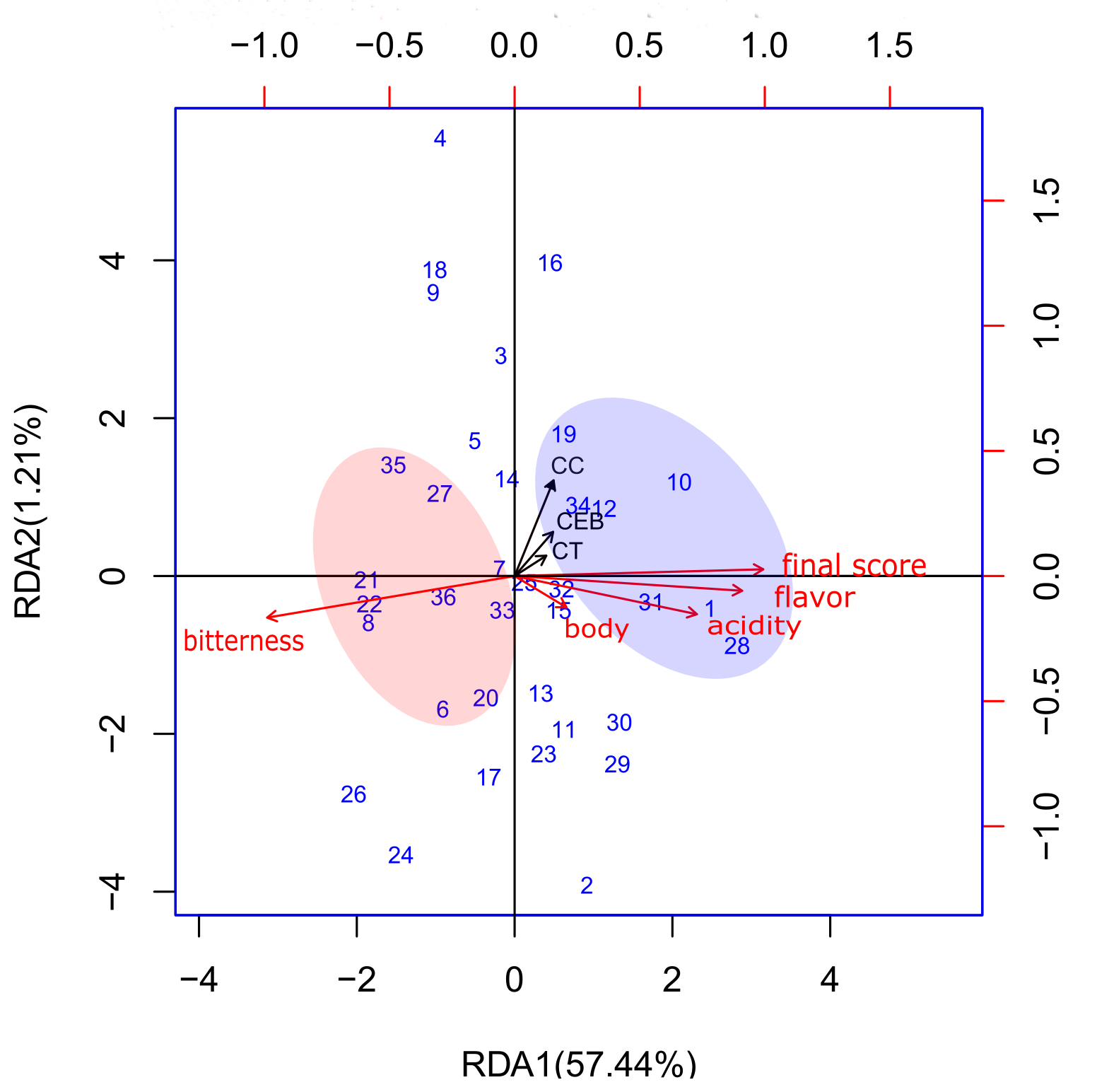 | 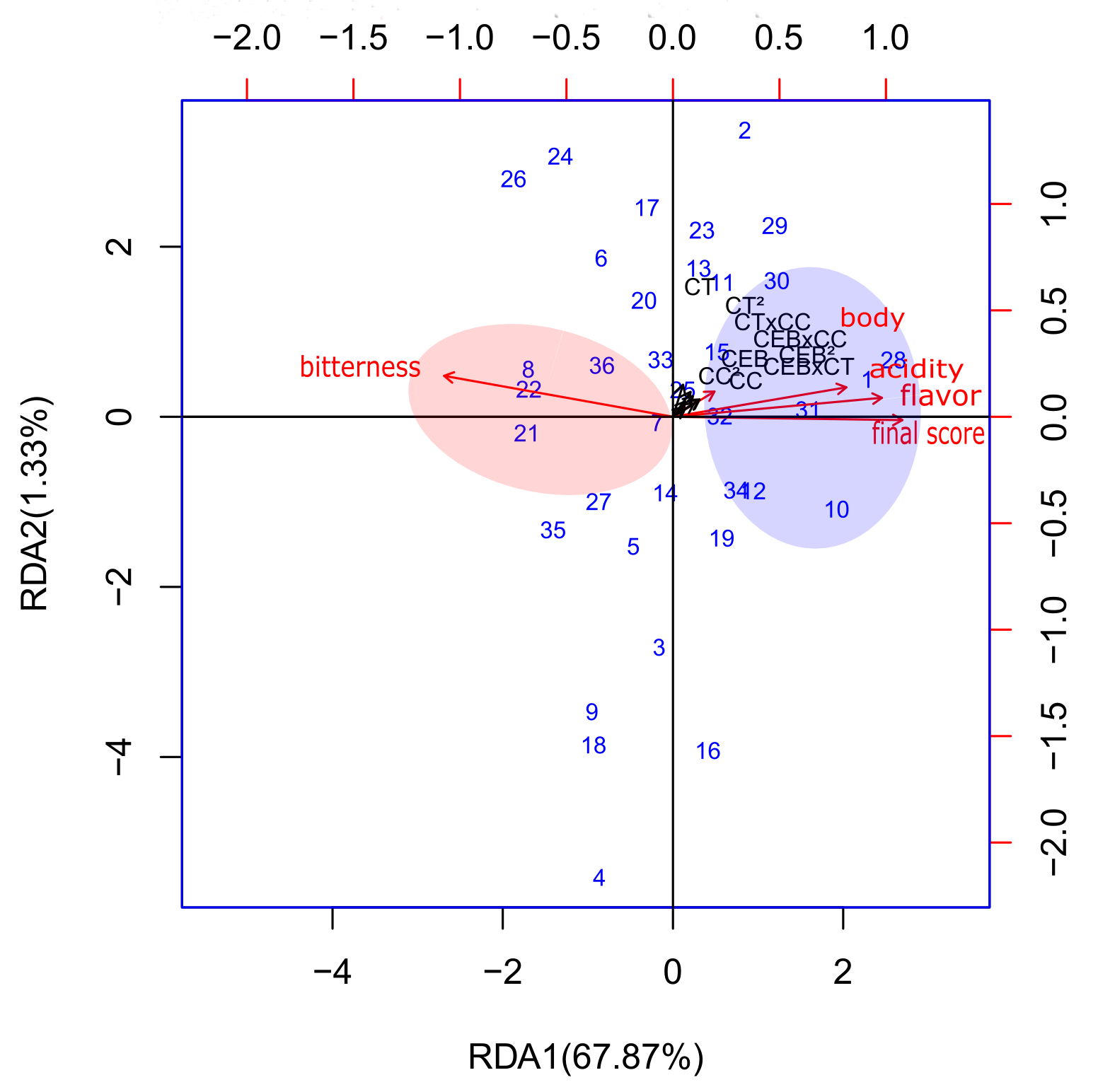 |
According to the triplot shown in Figure 1(a), two groups of samples can be considered: the first (in translucent blue) has samples associated with the sensory notes body, acidity, flavor and final score. In this group, pure coffee samples 1 and 28 stand out from the others, being closer to the maximum values of the sensory notes, especially for the attributes acidity, flavor and final score, while the samples of binary blends 15 and 32 are closer to the maximum values for body attributes. In the same group, but in the first quadrant, pure coffee sample 10 is distinguished from the other blends in the same quadrant, with the latter being mostly binary and ternary blends.
The second area grouped 10 samples of blends, defined by positive associations with the bitterness attribute; three samples (8, pure coffee; 21, a binary blend; and 22, a ternary blend) were strongly associated with intermediate values of the aforementioned attribute and three others (7, 33 and 36) with the same characteristics were strongly associated with lower values of bitterness. Therefore, it was concluded that within this group, it was not possible to observe significant differences between the pure coffee samples and the binary and ternary blends. Similar to the linear model, in Figure 1(b) of the polynomial model, the area in blue shows that pure coffee samples 1 and 28 are strongly associated with higher values of acidity, flavor and final grade and the coffee sample pure 10 moderately associated with higher final grade values, the difference is that for this model there was a quadrant inversion, where the first two now belong to quadrant I and the third to quadrant 4. In the red area, the samples belonging to the group remained the same, but the samples that were in quadrant III moved to quadrant II, displaced by the direction of the vector of the bitter attribute.
Canonical correspondence analysis
Similar to the previous section, Table 4 shows the main metrics used to evaluate the canonical correspondence analysis models.
| Linear CCA | ||||
|---|---|---|---|---|
| Transformation | Mean \(R^{2}\) | Var. Exp | Pseudo-F | Pseudo-F* |
| Chi-squared | 0.51 | 61.86 | 0.001 | - |
| ALR | 0.51 | 59.41 | 0.001 | - |
| CLR | 0.51 | 59.41 | 0.001 | - |
| ILR | 0.51 | 59.41 | 0.001 | - |
| Polynomial CCA | ||||
| Chi-squared | 0.63 | 69.00 | 0.001 | 0.300 |
| ALR | 0.66 | 72.34 | 0.001 | 0.025 |
| CLR | 0.67 | 71.77 | 0.001 | 0.036 |
| ILR | 0.66 | 70.54 | 0.001 | 0.058 |
Table 4 shows a configuration of results similar to those that occurred in the redundancy analysis, with the means of the coefficients of determination and explained variance for each approach showing that the results of the different transformations are very close.
All the models were significant, but only the models that used the additive log ratio and centered log ratio transformations justified the use of the polynomial approach, considering the fact that only these models were significant according to the pseudo-F test of the difference at the \(\alpha = 0.05\) level.
Considering these results, the linear model and polynomial model, for which data were subjected to the centered log ratio transformation, were considered because it was not necessary to forego a component to calculate the ratios for these data.
Centered Log-Ratio transformation
In the case of the models resulting from the Table 5, as well as in the models with the data transformed by the chi-square method, the linear approach produced three canonical axes, while the polynomial produced five axes, and the percentages of explained variance were 51.62% and 71.77%, respectively, for all the canonical axes.
| CCA | Canonical axes | ||||
| I | II | III | - | - | |
| Eigenvalues in relation to total variance | |||||
| 0.0334 | 0.0002 | 0.0000 | - | - | |
| Fraction of variance | |||||
| 59.0581 | 0.3509 | 0.0068 | - | - | |
| Fraction of accumulated variance | |||||
| 59.0581 | 59.4091 | 59.4160 | - | - | |
| Mean \(R^{2}\) | |||||
| 0.5162 | |||||
| PCCA | Canonical axes | ||||
| I | II | III | IV | V | |
| Eigenvalues in relation to total variance | |||||
| 0.03963 | 0.0005 | 0.0003 | 0.0001 | 0.0000 | |
| Fraction of variance | |||||
| 69.9326 | 0.9072 | 0.6597 | 0.2583 | 0.0152 | |
| Fraction of accumulated variance | |||||
| 69.9326 | 70.8398 | 71.4996 | 71.7579 | 71.7732 | |
| Mean \(R^{2}\) | |||||
| 0.6704 | |||||
| (a) | (b) | ||
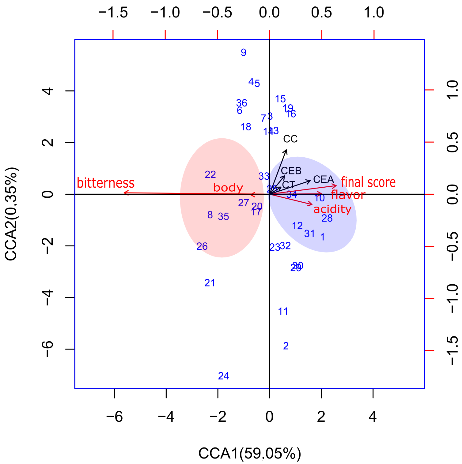 | 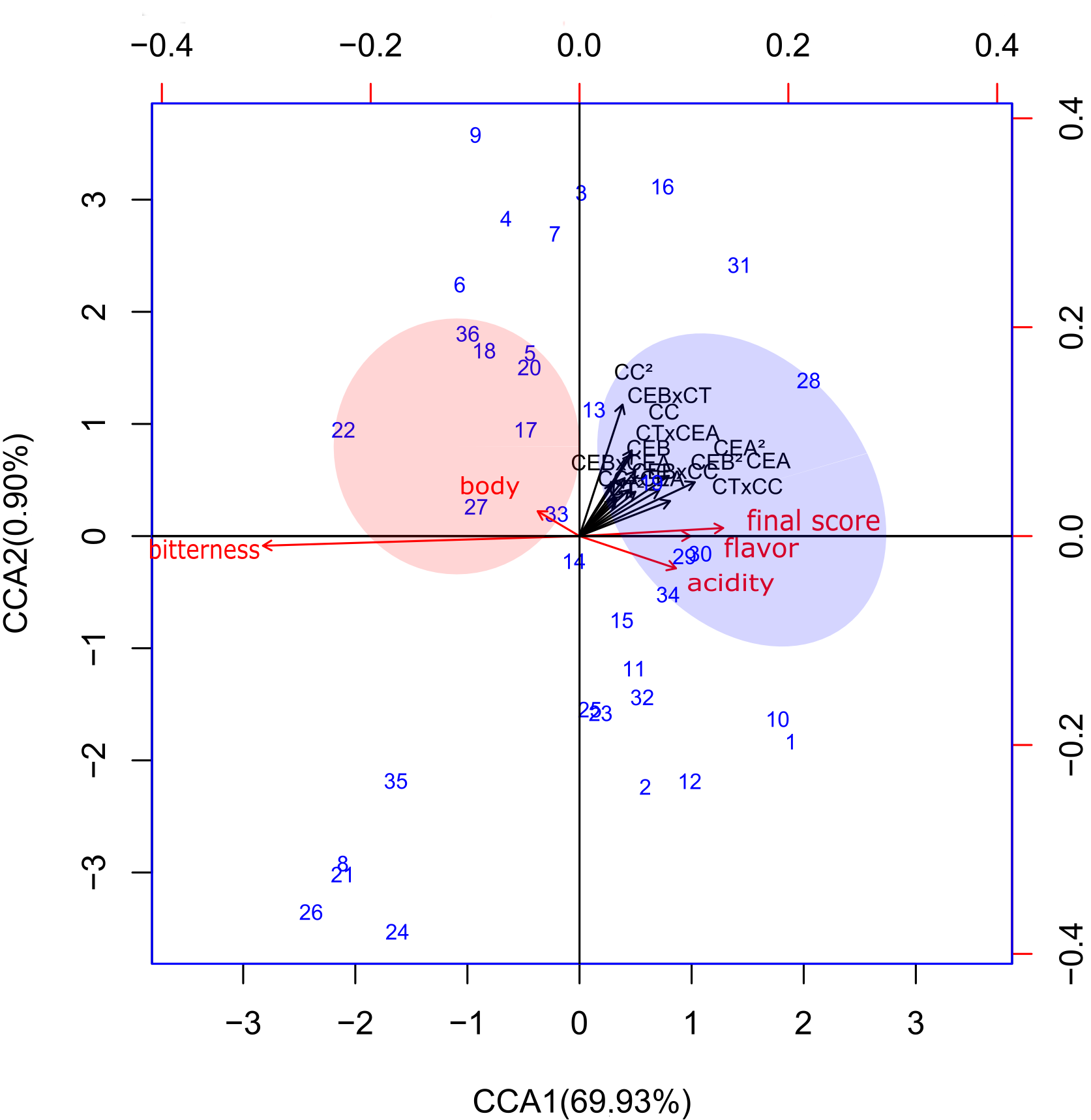 |
In Figure 2(a), the area in blue represents the aggregation of 7 samples, and the sample of pure Acaiá coffee 10 showed a strong association with the maximum values of the vectors representing the attributes flavor and acidity, whereas sample 28 of the same pure coffee showed a strong association with higher values of the acidity attribute but a smaller association with the flavor attribute, as did the sample of Bourbon Amarelo coffee, but with a slightly more moderate intensity of association.
In the same Figure 2(a), 7 samples are grouped in the area in red, where a sample of pure Conilon 27, a sample of pure commercial roasted coffee 17 and a sample of binary blend 20 were strongly correlated with higher scores for the body attribute. Nevertheless, the samples of the roasted commercial pure coffee 8 and 35 showed a strong association with intermediate values of the bitterness attribute, as did a binary blend (sample 22).
For the polynomial model, Figure 2(b), a greater dissimilarity between the pure coffee and the binary blend samples, shown in the blue area, was observed than in the classical linear model, given the greater distance between the samples. In this case, the binary 29 and ternary 30 blend samples showed strong correlations with higher values of the acidity and flavor attributes, while the binary sample 34 had a strong correlation with acidity and a moderate correlation with flavor.
A comparison of the results shown in the red areas of the plots for both approaches showed that binary sample 33 was more strongly associated with higher values for the body attribute, while the sample of pure Conilon 27 was separated from the samples of commercial pure roasted coffee 17 and binary blend 20.
Discussion
As the methodology used in this study involved several combinations of methods applied to the same database, it is appropriate to compare the performance of each method considering its purposes and particularities.
Regarding the transformations, it was noted that those derived from logarithmic ratios showed similar results, both in the mean of the coefficient of determination and in the percentage of explained variance. This was similar to the results found in Messias, 2016, who used these transformations of compositional data for the application of principal component analysis.
The three transformations derived from logarithmic ratios also produced biplots equivalent to each other, with the linear models having greater similarity than the polynomial models. This indicates that, as new variables are inserted into the models, there is greater dissimilarity in the results of these transformations, once again corroborating the findings of the study by Messias, 2016.
When comparing the logarithmic ratio transformations with the other transformation approaches, there was a small gain in the percentage of variance explained when the logarithmic ratio transformations were used in the linear redundancy analysis models. Conversely, in the polynomial redundancy analysis models, this gain was even greater, resulting in a significant difference according to the pseudo-F test. In the canonical correspondence analysis models, these differences were more subtle.
The biplots of the alr, clr and ilr models showed a grouping of the components in the first quadrant, while the standardization in the RDA and the chi square transformation resulted in these components having more dispersed coordinates throughout the graph.
In a theoretical and succinct sense, according to Legendre and Legendre & Legendre, 2012, the difference between redundancy analysis and canonical correspondence analysis is that in the first, linear regression is used to adjust the \(\mathbf{Y}\) values, while in the second, Y values are adjusted by means of weighted linear regression. That said, the solutions given by the canonical correspondence analysis differ very little from those given by the redundancy analysis, both in the evaluation metrics and in the biplots obtained, especially if we consider the use of log-ration transformations.
In most of the models constructed here, the polynomial approach provided a higher percentage of significant explained variance than the linear models. In general, in these cases, there is a greater relationship between the sensory notes and the interaction terms and quadratics of the blends. The same behavior was observed by Makarenkov & Legendre, 2002 in a study in which there was a significant gain in the explained variance in the distribution of spider species by quadratic terms and the interaction of environmental variables. In the triplots generated by these authors, most spider species were more associated with quadratic terms of the variables water, soil reflection and the interaction between water and soil reflection.
Regarding the sensory analysis of the blends, the conventional canonical correspondence analysis provided explained variance values close to 60%, which is considered reasonable in this type of analysis. The integration of terms that lead to a better quadratic approximation of the residuals through the polynomial algorithm led to a significant increase in the proportion of explained variance, with values greater than 70%. The polynomial modeling resulted in percentages consistent with those found in other studies, such as Costa et al., 2018, who obtained satisfactory results for the correspondence analysis using different distance metrics.
Regarding the triplots, it is worth noting that their interpretations are rather subjective, and it is up to the researcher to establish similarity criteria in relation to the distances between samples and variables. From this understanding, it follows that all the redundancy analysis models presented a pattern in which most of the samples were subdivided into two contrasting groups in the triplot. The first group was positively correlated with the attributes flavor, acidity, body and final score, and the second was positively correlated with the bitterness attribute.
Considering the isometric log-ratio polynomial model, in the first group, the samples of pure specialty Bourbon Amarelo and Acaiá coffees were not discriminated according to flavor or acidity because they had similar coordinates in the graph. Using mixed models to compare the effects of each component of the blends, Paulino et al., 2019 found the same results. Nevertheless, the blends could be discriminated from the other samples of pure coffees, with the points representing the binary and ternary blends being closer to the origin and up to half of the length of the arrows representing the attributes. This differentiation between the blending categories was also observed in Cirillo et al., 2019, who proposed a sensory panel of coffee blends based on the distribution of extreme scores.
In the second group, there was no differentiation between blending categories, but the samples that had a higher correlation with higher scores of the bitterness attribute included the roasted commercial coffee and lacked the Acaiá coffee. There is, therefore, evidence that commercial roasted coffee has less influence on Acaiá coffee than on the Bourbon Amarelo and Conilon coffees in relation to the bitterness attribute.
For the centered log-ratio polynomial model of the canonical correspondence analysis, the pure Bourbon Amarelo and Acaiá coffee samples were discriminated according to their concentrations: the samples with a concentration of 0.07 m/v were correlated with the acidity attribute, while the samples with a concentration of 0.10 m/v had a greater association with the attributes flavor and final score. The similarity between these two types of specialty coffees can be seen in Ossani et al., 2017 and justified by the genetic and environmental conditions of the coffees, such as altitude; in this case, the results show that the coffees were similar even at different concentration levels.
The second characteristic highlighted by this model, in addition to the bitterness attribute emphasized by the redundancy analysis, also was related to the body attributes and grouped other Conilon coffee samples that were not present in the redundancy analysis. According to Lima et al., 2015, certain varieties of Canephora coffee, such as Robusta, are used in the coffee industry for the formulation of blends in conjunction with specialty coffees because Robusta is more bitter and full-bodied, while specialty coffees are more fruity and acidic.
Conclusions
As demonstrated by the results of this study, the redundancy analysis and polynomial canonical correspondence analysis explained part of the variance in the sensory attribute scores that remained unexplained by the linear models.
Author contributions
H.S.P.T. Santos participated in the: Formal analysis, Programs, Methodology, Writing – Preparation of the original draft. M.A. Cirillo participated in the: Conceptualization, Formal analysis, Methodology, Supervision. F.M. Borém participated in the: Research, Resources. D.R. Fernández participated in the: Writing – proofreading and editing.
Conflicts of interest
The authors declare that there is no conflict of interest regarding the publication of this article.
Acknowledgments
The authors wish to thank the CAPES and CNPq \((N^{o} 140242/2019-8)\) - Brazil, for financial support.
References
Cirillo, M. A., Ramos, M. F., Borém, F. M., Miranda, F. M., Ribeiro, D. E., & Menezes, F. S. (2019). Statistical procedure for the composition of a sensory panel of blends of coffee with different qualities using the distribution of the extremes of the highest scores. 41(1), e39323. https://doi.org/10.4025/actasciagron.v41i1.39323
Costa, A. L. A. , Brighenti, C. R. G., & Cirillo, M. A. (2018). A new approach to simple correspondence analysis with emphasis on the violation of the independence assumption of the levels of categorical variables. e34953. https://doi.org/10.4025/actascitechnol.v40i1.34953
Costa, A. S., Resende, M., Nakayo, E. Y., Cirillo, M. A., Borém, F. M., & Ribeiro, D. E. (2020). Proposal of a metric selection index for correspondence analysis: an application in the sensory evaluation of coffee blends. 41(2), 479-492. https://doi.org/10.5433/1679-0359.2020v41n2p479
Ivoglo, M. G., Fazuoli, L. C. F., Oliveira, A. C. B., Gallo, P. B., Mistro, J. C., Silvrolla, M. B., & Toma-Braghini, M. (2008). Genetic divergence among robusta coffe progenies. 67(4), 823--831. https://doi.org/10.1590/S0006-8705200800040000
Lazraq, A., & Cléroux, R. (2002). Testing the significance of the successive components in redundancy analysis. 67(3), 411-419. https://doi.org/10.1007/BF02294993
Legendre, P., & Legendre, L. (2012). Numerical ecology. Elsevier.
Lima, T., Lucia, S. M. D., Saraiva, S. H., & Lima, R. M. (2015). Physico-chemical characterization of espresso coffee beverage prepared from blends of arabica and conilon coffees. 62(4), 333--339. https://doi.org/10.1590/0034-737X201562040001
Makarenkov, V., & Legendre, P. (2002). Nonlinear redundancy analysis and canonical correspondence analysis based on polynomial regression. 83(4), 1146--1161. https://doi.org/10.2307/3071920
Messias, R. M. (2016). Transformações em dados composicionais para a aplicação da análise de componentes principais.
Oksanen, A. J., Blanchet, F. G., & Kindt, R. (2020). Vegan: Community Ecology Package Version 2.5-7.
Ossani, P. C., Cirillo, M. A., Borém, F. M., Ribeiro, D. E. & Cortez, R. M. (2017). Qualidade de cafés especiais: uma avaliação sensorial feita com consumidores utilizando a técnica MFACT. 48(1), 92-100. https://doi.org/10.5935/1806-6690.20170010
Paulino, A. L. B., Cirillo, M. A., Ribeiro, D. E., Borém, F. M., & Matias, G. C. (2019). A mixed model applied to joint analysis in experiments with coffee blends using the least squares method. 50(3), 345--352. https://doi.org/10.5935/1806-6690.20190041
Rencher, A. C. (2002). Methods of multivariate analysis. John Wiley & Sons, Inc.
Ribeiro, B. B., Mendonça, L. M. V. L., Assis, G. A., Mendonça, J. M. A., Malta, M. R., & Montanari, F. F. (2014). Avaliação química e sensorial de blends de Coffea canephora Pierre e Coffea arabica L.. 9(2), 178--186.
Ribeiro, D. E., Borém, F. M., Cirillo, M. A., Prado, M. V. B., Ferraz, V. P., Alves, H. M. R., & Taveira, J. H. S. (2016). Interaction of genotype, environment and processing in the chemical composition expression and sensorial quality of Arabica coffee. 11(27), 2412--2422. https://doi.org/10.5897/AJAR2016.10832
Stewart, D., & Love, W. (1968). A general canonical correlation index. 70(3), 160--163. https://doi.org/10.1037/h0026143
Ter Braak, C. J. F. (1986). Canonical correspondence analysis: a new eigenvector technique for multivariate direct gradient analysis. 67(5), 1167--1179. https://doi.org/10.2307/1938672
Wickham, H., François, R., Henry, L., Muller, K., & Vaughant, D. (2020). dplyr: A Grammar of Data Manipulation.
Van den Wollenberg, A. L. (1977). Redundancy analysis an alternative for canonical correlation analysis. 42(2), 207--219. https://doi.org/10.1007/BF02294050