
Stability of the Epidemiological Model SIR with Loss of Immunity
Ferreira, A. L; Araujo, K. B. G.
DOI 10.5433/1679-0375.2023.v44.47860
Citation Semin., Ciênc. Exatas Tecnol. 2023, v. 44: e47860
Abstract:
This study approaches the analysis of the stability of the epidemiological model SIR with loss of immunity. This is a model given by a system of ordinary differential equations. Initially, we present the model and its interpretation. Then we define the constants and elements that compose the model, so we present the results obtained using the qualitative theory of ordinary differential equations, especially the theory of planar systems related to the dynamics of fixed points. Finally, we show that the system representing the SIR model is globally stable and they have two types of dynamic that depend on model constants, and their meaning for epidemiology.
Keywords: SIR model, ordinary differential equations, fixed points, stability
Introduction
Ordinary differential equations are widely used for modeling real-world problems such as population growth, species interactions, physical phenomena, epidemics, and others (Zill, 2003).
In particular, epidemic models are extensively used as they aid in predicting and understanding how a disease spreads, and the duration of an epidemic and help the implementation of methods to reduce the disease’s impact on the population. These models are highly efficient in determining the best control measures, which depend on the disease, population, and epidemic scale. However, these models have limitations, such as their inability to precisely predict which portions of the population will be infected or the exact course of the epidemic (Keeling & Rohani, 2008).
It is estimated that mathematical studies on diseases began more than 300 years ago, given the various epidemics that have occurred in the world. The first mathematical model for an epidemic was developed by Daniel Bernoulli (1700-1782) to study and show that inoculation with a live virus obtained from a patient of smallpox, would reduce the death rate and increase the population of France, see Daley & Gani, 2001 for more details. With the formalization of epidemiological mathematics in conjunction with biologists and physicians various advances have been made in the study of epidemics, such as studies on Malaria by Ross, 1911 and the studies by Kermack & McKendrick, 1927 which were landmarks for epidemiological studies (Shil, 2016).
In this study, we consider an acute infectious disease, meaning a disease that manifests itself over a short period of days or weeks, such as influenza, flu, and chickenpox. We study the compartmental SIR model by Kermack & McKendrick, 1927, which divides a population into compartments and shows how the numbers in these compartments may fluctuate over time. For simplification, we consider a closed population without demography and the factor of the individuals losing immunity after a certain period of time (Keeling & Rohani, 2008). We use results from the Qualitative Theory of Ordinary Differential Equations present in Doering & Lopes, 2016, Sotomayor, 2011, Arrowsmith & Place, 1982, and Perko, 2013, to do the same as Báez-Sánchez & Bobko, 2020 for our simplified model, that is, study the stability of this model in relation to its parameters, since the focus is the dynamic of the system. This type of study is very important since the dynamic of the system helps to predict how the disease spreads the population. An example of this is the use of the SIR model for COVID-19, and it can be seen in [Nesteruk2021 - not found].
Materials and methods
First let us define the SIR model proposed by Kermack & McKendrick, 1927. Consider the population is fixed and the individuals are homogeneously mixed. S(t) represents the fraction of susceptible individuals at time t, I(t) is the fraction of infected individuals at time t, and R(t) is the fraction of recovered individuals at time t given by
(1)
S(t)+I(t)+R(t)=1. In equation (1), the susceptible are the individuals who can become infected, the infectious are individuals who have the disease and we assume that while they have the disease they are capable of infecting susceptible individuals and the recovered are the individuals who have recovered from the disease. This model we add the assumption that recovered individuals lost their immunity to the disease after a certain period of time.
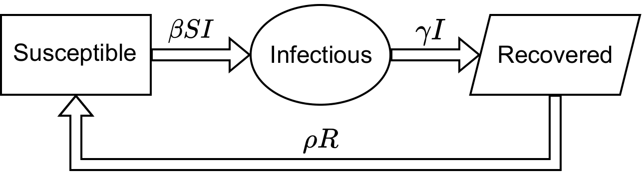
A susceptible individual contracts the disease from an infectious individual at a rate β>0, thus becoming infected and staying infected until it recovers at a rate γ, so this recovered individual becomes susceptible again at a rate ρ. The model is given by equations (2)-(4),
(2)
S′=−βSI+ρR,
(3)
I′=βSI−γI,
(4)
R′=γI−ρR,
where (′) represents the time derivative and the system is subject to the initial conditions.
We are considering the individuals move between the compartments following the diagram presented in Figure 1.
Constant β
Using the law of mass action in epidemiology, we assume that the disease spreads at a rate proportional to the product of the fractions of susceptible and infectious populations, considering that individuals randomly encounter it (Pachi, 2006). Therefore, as defined in López-Flores et al., 2021, we define the proportionality constant β as the product of the average number of individuals contacted by an infected individual per day and the probability of transmission, and is called transmission coefficient, which indicates the rate of new infections when a contact occurs between susceptible and infected individuals.
Constant γ
We can define the constant γ as in López-Flores et al., 2021, based on the concept of probability distribution. For this purpose, we assume the entire population is infected at t=0, i.e, I(0)=1, and there are no new infections, then βSI=0, thus from equation (3) we isolate the recovery phenomenon, so we get
(5)
{I′=−γII(0)=1.
The analytic solution of the system described by equation (5) is
(6)
I(t)=e−γt.
By deriving equation (6), we have the rate at which I(t) varies, so
(7)
I′=−γe−γt.
The rate represented by equation (7) is negative, as I(t) is decreasing because people recover over time. The equation (7) also represents the rate at which people recover and when we take −I′(t) it is a positive rate, given by a fraction of the population per unit of time. When everyone recovers, we have
(8)
∫∞0−I′dt=∫∞0γe−γtdt=−e−γt⏐
therefore, with equation (8) and -I'\geq 0, we have that -I'(t) is a probability density function for 0\leq t < \infty. The average time that individuals are with the disease is given by the mean, or expected, value of t in this interval, that is,
\begin{aligned} \int_{0}^{\infty}t(-I')dt = \int_{0}^{\infty}\gamma te^{-\gamma t}dt = \dfrac{1}{\gamma}. \end{aligned}
Thus, we can interpret \gamma as the rate at which individuals recover, and \frac{1}{\gamma} as the average time individuals stay with the disease and its unit being 1/\text{day}.
Constant \rho
In the same way as we did for the constant \gamma, we assume at t=0 the entire population is recovered, that is, R(0) = 1 and don’t have new infectious, i.e, \gamma I=0. From equation (4) we can isolate the phenomenon of losing immunity and obtain,
(9)
\begin{aligned} \begin{cases} R'=-\rho R\\ R(0) = 1. \end{cases} \end{aligned}
The analytic solution of the system described by equation (9) is
(10)
\begin{aligned} R(t) = e^{-\rho t}. \end{aligned}
By deriving equation (10), we have
(11)
\begin{aligned} R'=-\rho e^{-\rho t}, \end{aligned}
which is negative, as R(t) decreases because individuals lose their immunity over time and become susceptible again. From equation (11), we have -R'=\rho e^{-\rho t}, which is positive and indicates the rate of individuals that lose their immunity and is measured by a fraction of the population per unit of time. So, when all individuals become susceptible again we have
(12)
\begin{aligned} \int_{0}^{\infty}-R'dt = \int_{0}^{\infty} \rho e^{-\rho t} dt = -e^{-\rho t}\Big\arrowvert_{0}^{\infty} = 1. \end{aligned}
Therefore, since -R'(t)>0 and equation (12) holds, -R' is a probability density function for 0\leq t < \infty. Thus the average time that individuals remain immune is given by \begin{aligned} \int_{0}^{\infty}t(-R')dt = \int_{0}^{\infty}\rho te^{-\rho t}dt = \dfrac{1}{\rho}, \end{aligned} so \rho its the rate at which individuals become susceptible again, and the average time until they lose their immunity is \dfrac{1}{\rho}, which is given by 1/\text{day}.
Basic reproductive ratio
Let’s define now the basic reproductive ratio, as in Keeling & Rohani, 2008, denoted by R_0. This is a very important value in epidemiological models. It is the average number of individuals infected by each infectious individual when a disease is introduced into the population, that is, it gives us the number of individuals that each infectious individual can infect, assuming that the entire population is susceptible to the disease. We can represent it as,
(13)
\begin{aligned} R_0 = \beta \dfrac{1}{\gamma} = \dfrac{\beta}{\gamma}. \end{aligned} We are looking at each infectious individual and calculating how many susceptible individuals can transmit the disease during the time they are infected. For example, Table [tab1] shows estimated values of R_0 for different diseases.
| Disease | R_0 | Source |
|---|---|---|
| Influenza | 1.2-1.4 | Chowell et al., 2008 |
| Chickenpox | 10-12 | Zaparolli, 2020 |
| SARS | 2-4 | World Health |
| Organization (2003) |
Using the equation (1), we have R=1-S-I, so we can rewrite the equations (2) and (3) by
(14)
S'=-\beta SI + \rho(1-S-I),
(15)
I'=\beta SI - \gamma I.
We will analyze the stability of the equations (14) and (15) in the phase plane given by \mathcal{T} = \{(S,I): S\geq 0,\, I\geq 0,\, S + I \leq 1 \}, which is a compact set.
Results and discussion
From the definition and representation (13) of R_0 we can note:
If R_0>1 the disease will spread in the population;
If R_0<1 the disease will not spread in the population.
This already shows the importance of this value, as if we have a very high R_0, the disease spreads quickly through the population. And from its definition, we can introduce measures that help to decrease the value of R_0, if we can change the constants \beta and \gamma.
In this context, we will analyze the dynamics of the system described by equations (14) and (15) for R_0>1 and R_0<1.
Local stability
For a local stability analysis, first we will find the nullclines for the system, that is, when
(16)
S'=-\beta SI + \rho(1-S-I)=0,
(17)
I'=\beta SI - \gamma I=0,
with equations (16) and (17) we have
S'=0 when I=\dfrac{\rho - \rho S}{\rho + \beta S};
I'=0 when I=0 or S=\dfrac{\gamma}{\beta}.
The fixed points, or equilibrium points, are when S' and I' are zero and in this case we have two fixed points, given by (S_*,I_*) = (1,0) and (S_e,I_e)= \left( \dfrac{\gamma} {\beta},\dfrac{\rho(\beta-\gamma)}{\beta(\rho+\gamma)}\right).
Note that, when R_0 < 1, we have \dfrac{\gamma}{\beta}>1, so the fixed point (S_e,I_e) will not be in the phase plane. We can graphically see where these fixed points are located in the phase plane for both cases.
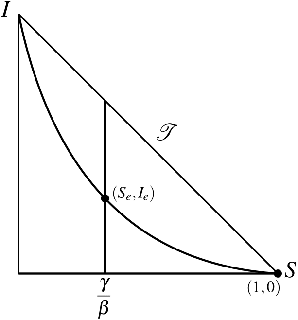
Figures 2 and 3 show the nullclines and fixed points for R_0<1 and R_0>1, respectively.
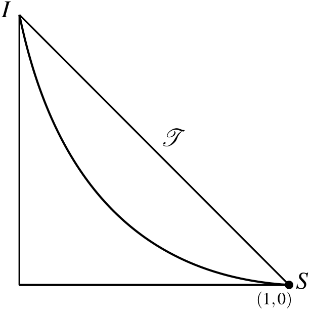
In Figure 2, we can observe the nullclines of S and I in the phase plane \mathcal{T} for R_0<1. In this case, there exists a unique fixed point in \mathcal{T}, which is (S_*,I_*).
In Figure 3, we have the nullclines of S and I in the phase plane \mathcal{T} for R_0>1. In this case we have (S_*,I_*) and (S_e,I_e) in \mathcal{T}.
The system, equations (14) and (15), is not a linear system. Therefore, for the study of its local stability, we perform a linearization of the system. This involves studying the Jacobian matrix of the system, which is
(18)
J(S,I)= \left( \begin{array}{cc} -\beta I - \rho & -\beta S - \rho \\[0.35cm] \beta I & \beta S - \gamma \end{array} \right). The trace (\tau) and determinant (\Delta) of J are relative with the eigenvalues of the matrix in equation (18) (Sotomayor, 2011), thus:
For the fixed point (S_*,I_*) we have the matrix,
(19)
J(S_*,I_*) = \left( \begin{array}{cc} - \rho & -\beta - \rho \\[0.35cm] 0 & \beta - \gamma \end{array} \right), we have the trace and determinant is,
(20)
\tau = (-\rho + \beta - \gamma),
(21)
\Delta = -\rho(\beta - \gamma).
For the fixed point (S_e,I_e) we have the matrix,
(22)
J(S_e,I_e) = \left( \begin{array}{cc} - \rho\dfrac{\beta-\gamma}{\rho + \gamma} -\rho & -\gamma - \rho \\[0.5cm] \rho\dfrac{\beta-\gamma}{\rho + \gamma} & 0 \end{array} \right), where,
(23)
\tau = - \rho\dfrac{\beta-\gamma}{\rho + \gamma} -\rho,
(24)
\Delta = \rho(\beta - \gamma).
The matrices (19) and (22) show us that:
If R_0<1, we only have the fixed point (S_*,I_*) inside the phase plane, and in this case from equations (20) and (21) we have, \Delta>0 and \tau < 0. Thus (S_*,I_*) is an attractor for the linear system given by the matrix in equation (18), and by the Lyapunov-Perron Theorem (Doering & Lopes, 2016), it is also an attractor for the nonlinear system described by equations (14) and (15). This means that all solutions that start close to it in the phase plane will approach it as time increases.
If R_0 > 1, we have both fixed points in the phase plane. For (S_*,I_*), from equation (21), we have \Delta~< 0, so it is a saddle point for the linear system given by the matrix in equation (18), meaning that solutions starting outside of this equilibrium will move away from it. By the Linearization Theorem (Arrowsmith & Place, 1982), (S_*,I_*) is also a saddle point for the system described by equations (14) and (15). For (S_e,I_e), with equations (23) and (24), we have \Delta > 0 and \tau < 0, so it is an attractor by the matrix, equation (18), and, by the Lyapunov-Perron Theorem (Doering & Lopes, 2016), (S_*,I_*) is a saddle point, and (S_e,I_e) is an attractor for the system, equations (14) and (15).
The Linearization and Lyapunov-Perron Theorems give us the dynamics of solutions locally around each fixed point. So, locally, when the disease is not spreading in the population, the system will approach (S_*,I_*) = (1,0), meaning that there will be no infectious individuals and the entire population will be susceptible. Now, when the disease is spreading, given an initial condition close to (S_e,I_e), the solutions will move away from (S_*,I_*) and tend for (S_e,I_e), which means that we will always have a fraction of the population of infectious individuals, and in epidemiology, this value is called the endemic equilibrium.
Global Stability
In the study of global stability, we want to determine what happens to solutions that start in the phase plane but are far from the fixed points.
We initially have that solutions starting at I=0 remain at I=0 and approach (S_*,I_*), since I=0 is the stable manifold of that fixed point. To analyze solutions starting at other points, we will use the differentiable function V:\mathcal{T} \to \mathbb{R}, given by V(S,I)=S+I. We have that V(S(t),I(t)) gives us the value of V along the solutions of equations (14) and (15) (Perko, 2013), and we are analyzing solutions on the line S+I=1. From this, we have, \begin{aligned} \langle \nabla V(S,I), (S',I')\rangle = \rho(1-(S+I)) - \gamma I \leq 0, \end{aligned} for S+I = 1, i.e, solutions that start on this boundary of the phase plane will continue on the phase plane. We now need to verify that they approach the equilibrium (S_e,I_e).
By the Poincaré-Bendixon Theorem (Sotomayor, 2011), as the solution remains in a compact set, it will approach either an fixed point or a closed orbit. We will use the Dulac’s Criterion (Doering & Lopes, 2016) for the open set E=\{(S,I) \in \mathbb{R}^2, I>0\} that has no holes and the differentiable function g:E \to \mathbb{R}, given by g(S,I) = \dfrac{1}{I}. Thus,
(25)
\begin{aligned} \text{div}(g(S,I)S',g(S,I)I') = -\beta - \dfrac{\rho}{I}, \end{aligned}
since the divergence, equation (25), does not change sign and is not zero for I>0, we do not have closed orbits in this open set. Therefore, solutions start in the phase plane will only approach the fixed point.
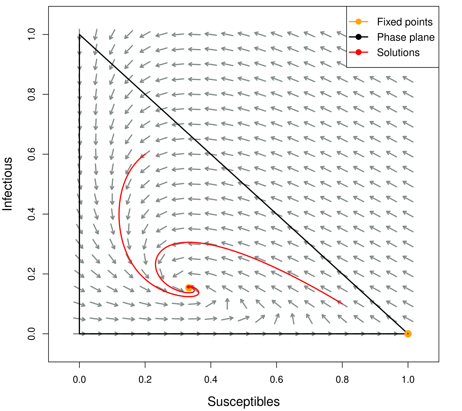
Using the programming language R and modified codes from (Frost et al., 2018), we computed the vector fields for the SIR model by assigning values to the parameters. In Figures 4 and 5, we can visualize the results obtained from the stability analysis of the model.
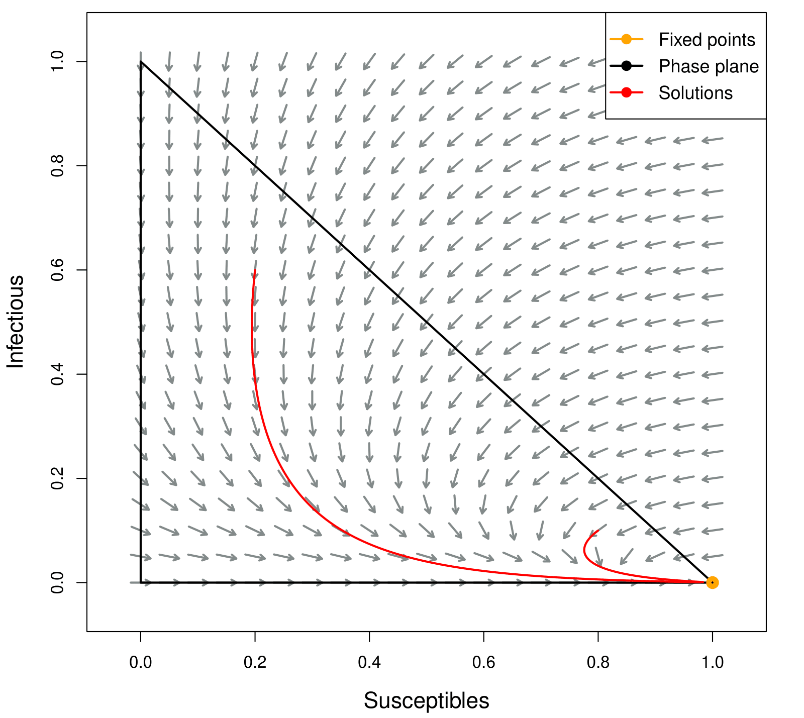
In Figure 4 we have a disease in which people stay sick for an average of 8 days, and remain immune for an average of 30 days and the transmission coefficient is 0.1, that is, a 10% probability of transmission in contact between infected and susceptible. Therefore, we have R_0<1, and the solutions will converge to the point (S_*,I_*). The simulation used initial conditions of S_0=0.2, I_0=0.6 and S_0=0.8, I_0=0.1.
In Figure 5 we have a simulation for a disease with R_0>1, i.e, is spreading through the population. In this case individuals stay sick for around 10 days, remain immune for an average of 30 days and the transmission coefficient is 0.3, that is, a 30% probability of transmission in contact between infected and susceptible. As we can see, the solutions converge to the fixed point (S_e,I_e). The initial conditions used were S_0=0.2, I_0=0.6 and S_0=0.8, I_0=0.1.
Conclusions
We can conclude that the SIR model with loss of immunity is stable, regardless of its parameters and for both cases of R_0. However, for each case, we have different behaviors of the system dynamics. We have:
For R_0 < 1, the disease does not spread, and all solutions converge to the equilibrium point of the phase plane, where the number of infected individuals in the population is zero.
For R_0 > 1, the solutions approach the endemic equilibrium, which indicates that for a disease with these assumptions, we will always have infectious individuals within the population. Consequently, the disease will always be present in the population at the endemic equilibrium.
In addition, we have an estimate of the number of individuals in each compartment for the system to reach equilibrium, which is a value sought when studying the spread of a disease over a long period of time. This study also shows that it is possible to introduce control factors, and methods that decrease the \beta constant, thus modifying the R_0 and making the spread of the disease smaller, reducing its impact within the population. For example, the controlling factor can be using masks or control the encounter of the susceptible with the infectious.
Author contributions
A.L. Ferreira participated in the: Conceptualization, Methodology, Supervision, Writing - Revision. K.B.G. Araujo participated in the: Data curation, Research, Writing - Original Draft, Revision and Editing.
Conflicts of interest
The authors declare no conflict of interest.
Acknowledgments
The second author would like to thank the Secretaria de Educação Superior (SESu) of the Ministério da Educação (MEC) and the National Fundo Nacional de Desenvolvimento da Educação (FNDE) for the Bolsa PET, which funded this project.
References
Arrowsmith, D. K., & Place, C. M. (1982). Ordinary differential equations: A qualitative approach with applications. Chapman and Hall.
Báez-Sánchez, A. D., & Bobko, N. (2020). On equilibria stability in an epidemiological sir model with recovery-dependent infection rate. TEMA, 21, 409–424. https://doi.org/10.5540/tema.2020.021.03.0409
Chowell, G., Miller, M., & Viboud, C. (2008). Seasonal Influenza in the United States, France, and Australia: Transmission and Prospects for Control. Epidemiology & Infection, 136(6), 852–864. https://doi.org/10.1017/S0950268807009144
Daley, D. J., & Gani, J. (2001). Epidemic Modelling: An Introduction. Cambridge University Press.
Doering, C. I., & Lopes, A. O. (2016). Equações Diferenciais Ordinárias. Editora do IMPA.
Frost, S., Walsh, A., & Thompson, J. (2018). Epirecipes: A Cookbook of Epidemiological Models. http://epirecip.es/epicookbook/chapters/simple
Keeling, M. J., & Rohani, P. (2008). Modeling Infectious Diseases in Humans and Animals. Princeton University Press.
Kermack, W. O., & McKendrick, A. G. (1927). Contributions to the Mathematical Theory of Epidemics, Part I. Proceedings of the Royal Society of London, 115, 700–721.
López-Flores, M. M., Marchesin, D., Matos, V., & Schecter, S. (2021). Equações Diferenciais e Modelos Epidemiológicos. Editora do IMPA.
Pachi, C. G. F. (2006). Modelo Matemático para o Estudo da Propagação de Informações por Campanhas Educativas e Rumores [Dissertation, Universidade de São Paulo]. Universidade de São Paulo.
Perko, L. (2013). Differential Equations and Dynamical Systems (Vol. 7). Springer Science & Business Media.
Ross, R. (1911). The Prevention of Malaria. John Murray.
Shil, P. (2016). Mathematical Modeling of Viral Epidemics: A Review. Biomedical Research Journal, 3(2), 195–215.
Sotomayor, J. (2011). Equações Diferenciais Ordinárias. Editora Livraria da Física.
World Health Organization. (2003). Consensus Document on the Epidemiology of Severe Acute Respiratory Syndrome (SARS). World Health Organization. https://apps.who.int/iris/handle/10665/70863
Zaparolli, D. (2020). O Desafio de Calcular o R. Pesquisa FAPESP, 293, 46–47. https://revistapesquisa.fapesp.br/o-desafio-de-calcular-o-r/
Zill, D. G. (2003). Equações Diferenciais com Aplicações em Modelagem. Cengage Learning Editores.
Nesteruk, I. (2021). The real COVID-19 pandemic dynamics in Qatar in 2021: simulations, predictions and verifications of the SIR model. Semina: Ciências Exatas e Tecnológicas, 42(1Supl), 55–62. https://doi.org/10.5433/1679-0375.2021v42n1Suplp55