
Quality Parameter for Edge Representation of Images via Cubic Spline
Cirilo, E. R.; Figliaggi, B. R. M.; Natti, P. L.
DOI 10.5433/1679-0375.2023.v44.47720
Citation Semin., Ciênc. Exatas Tecnol. 2023, v. 44: e47720
Abstract:
This paper presents a new quality parameter for edge generation of two-dimensional images via spline interpolation. The motivation of the study is to define a parameter which allows establishing a stop criterion for inserting image data and obtaining a representation via spline that is sufficiently faithful. The parameter is deduced by an iterative calculation process between areas limited by cubic and linear splines after insertion of points. Then, after convergence, the parameter qualifies the fidelity of the computational representation of the image. The numerical code is developed from the octave software, and some images were generated validating the new parameter.
Keywords: quality parameter, spline, interpolation, image representation, octave
Introduction
The interpolation technique by spline is widely used as a tool for digital image processing/imaging.
The imaging is associated with computational algorithms that allow recognition or reconstruction of boundaries, improvement of image, quality and other aspects (Fadnavis, 2014). In this context, spline is a technique of interpolation that allows the reconstruction of boundaries, as it is seen in the work of Saita et al., (2017), in which the outline of Luruaco Lake (Colombia) was computationally implemented by cubical splines.
The technique can be utilized in improving images as it is seen on the works of Enjilela et al., (2019) and Zachariadis et al., (2019), that splines are used as auxiliary techniques in a reconstruction algorithm of tomography.
In this work, it is shown the cubic spline, a particular case of B-spline, as a data interpolation method to obtain images. This method can be implemented by a computational algorithm, that is not too complex (Habermann & Kindermann, 2007; Enjilela et al., 2019) and that presents a better performance on the interpolation. Furthermore, this technique is recommended for a data set with a large amount of knots, considering that it avoids unwanted oscillations (Ruggiero & Lopes, 1997), something that could occur in the reconstruction of complex geometries, in other words, geometries with a lot of details how can be seen at the famous Tarsila do Amaral’s paint, as shown in Figure 1(a), along with its corresponding representation using splines, depicted in Figure 1(b).
| (a) |
 |
| (b) |
 |
Therefore, the objective of this work is to present a method aligned to spline interpolation that generates the edge of any complex two-dimensional image as close as possible to the original image, in which most details are preserved in the computational representation. Furthermore, specifically it presents a brand new parameter of quality, which indicates the detailing of computational reconstruction by spline interpolation.
The article was organized in the following way: The methods of interpolation by spline linear and cubic were defined and discussed, emphasizing the importance of comprehending the initial impositions for the cubic splines (Ruggiero & Lopes, 1997). We emphasize that the representations of two-dimensional geometries shown in this work were created based on the parameterization of the data, which makes it possible to generate strict monotonicity curves. This is the code that we developed to number the data, therefore, we are always guaranteed to be computing coefficients of interpolating functions. Furthermore, next, we approached various mathematical techniques that support the definition of the new quality parameter for the representation by cubic splines.
We emphasize that all procedures that were mathematically modeled were implemented through the free software octave (Eaton et al., 2022).
For a didactic explanation, some images more simpler than Tarsila do Amaral’s paint were generated, and the discussions were presented in such a way to demonstrate quantitative and qualitative forms of the final representations.
Materials and methods
Spline
Spline is a form to interpolate a tabulated function \(f\) in each sub-range \([x_i,x_{i+1}],i=1,\cdots n\) by a degree of a polynomial \(p\). Thereby, we consider the idealized function in the Table 1.
| \(x\) | \(x_1\) | \(x_2\) | \(\cdots\) | \(x_{n}\) | \(x_{n+1}\) |
|---|---|---|---|---|---|
| \(f(x)\) | \(y_1\) | \(y_2\) | \(\cdots\) | \(y_{n}\) | \(y_{n+1}\) |
The function, \(S_p(x)\), of \(p\) degree, is a spline that has to satisfy the following criteria:
be a degree of a polynomial \(p\) in each sub-range \([x_{i},x_{i+1}]\), \(i=1,...,n\);
be continuous and have derived until the order \((p-1)\) in \([x_1,x_{n+1}]\);
\(S_p(x_i)=f(x_i)\), \(i=1,...,n+1\).
Notice that spline is a piecewise polynomial function, so increasing the number does not cause an increase in the degree of polynomial interpolation. Instead, the degree is defined prior to the interpolation (Ruggiero & Lopes, 1997).
Linear spline function
One of the particular cases of splines is the linear ones (\(S_1\)), in which they are formed by polynomials of first degree, in particular the linear spline functions will be indicated by \(SL\). By such means, given a function \(f\) as shown in the Table 1, the interpolating linear splines from \(f\) are defined by equation (1)
(1)
\[ SL(x) = \begin{cases} SL_1(x), \,\, &x \in [x_1,x_2]\\ \vdots\\ SL_{n}(x), \,\, &x \in [x_n,x_{n+1}] \end{cases}\]
where each polynomial \(SL_k(x)=m_k \cdot x+l_k\) such as
\[m_k = \dfrac{ y_{k+1} - y_k}{ x_{k+1}-x_{k} }\ \ and \ \ l_k = \dfrac{ (y_{k} \cdot x_{k+1}) - (y_{k+1} \cdot x_{k}) }{ x_{k+1}-x_{k} }\]
with \(k=1, \cdots ,n.\)
Cubic spline function
Another particular case of splines is cubic splines functions (\(S_3\)) which will be denominated by \(SC\). Therefore, considering \(f\), with values according to the Table 1, the function \(SC\) is defined by
(2)
\[ SC(x) = \begin{cases} SC_1(x), &x \in [x_1,x_2]\\ \vdots\\ SC_{n}(x), &x \in [x_n,x_{n+1}] \end{cases}\]
each polynomial is explictly written by \(SC_k(x)=a_k(x-x_k)^3+ b_k(x-x_k)^2+c_k(x-x_k)+d_k\), with \(k=1, \cdots ,n\).
Apart from fulfilling the three criteria mentioned, the polynomial \(SC_k(x)\), equation (2), also needs to satisfy the following conditions:
\(SC_k(x_k)=SC_{k-1}(x_{k})\), \(k=2,\cdots, n\);
\(\dfrac{d}{dx}SC_k(x_k) = \dfrac{d}{dx}SC_{k-1} (x_{k})\), \(k=2,\cdots, n\);
\(\dfrac{d^2}{dx^2}SC_{k} (x_{k}) =\dfrac{d^2}{dx^2}SC_{k-1} (x_{k})\), \(k=2,\cdots, n\).
Observe that the cubical spline \(SC_k(x)\) has the first and second continuous derivatives. In that way, the graph does not show sudden changes in curvature (Ruggiero & Lopes, 1997). In other words, there is smoothness in the meeting between splines through the knots in \(x_k\).
Notice that to calculate the interpolating cubical spline is necessary to determine the value of each coefficient \(a_k, b_k, c_k\) and \(d_k\) of the polynomials \(SC_k(x)\). On the work of Figliaggi and Cirilo (2021) is presented the deductions of coefficients, that take the following form: \(a_k=\dfrac{g_{k+1}-g_{k}}{6h_{k}}\), \(b_k= \dfrac{g_{k+1}}{2}\), \(c_k=\dfrac{y_{k+1}-y_{k}}{h_{k}}+\dfrac{(2g_{k+1}+g_{k})h_{k}}{6}\) and \(d_k=y_k\)
in which \(f(x_k)=y_k\), \(g_k = \dfrac{d^2}{dx^2}SC_{k} (x_{k})\), \(g_{k+1} = \dfrac{d^2}{dx^2}SC_{k+1} (x_{k+1})\) and \(h_k=(x_{k+1}-x_{k})\), for \(k=1,\cdots, n\).
The terms of the second derivative are labeled as \(g\), with \(k=1,\cdots,n+1\), and are calculated by the system
(3)
\[ \begin{cases} h_2g_{1}\!+2(h_{3}+h_2)g_2+h_{3}g_{3} = 6 M_2\\ \vdots\\ h_{n}g_{n-1} \!+\!\! 2(h_{n+1}\!+\!h_{n})g_{n}\!\!+\! h_{n+1}g_{n+1} = 6 M_{n} \end{cases}\]
in which \(M_k = \dfrac{y_{k+1} - y_{k}}{h_{k+1}} - \dfrac{y_{k}-y_{k-1}}{h_{k}}\), \(k=2, \cdots ,n\).
It is easy to see that the system, given in equation (3), does not have a number of equations equal to the number of unknowns. Therefore, it is necessary to impose auxiliary conditions for the system to have only one solution. The most important ones, and the most common conditions are:
Natural – imposing \(g_1=g_{n+1}=0\);
Approximation by parabola – imposing \(g_1=g_2\) and \(g_{n}=g_{n+1}\), which implies not changing the concavity of the extreme polynomials of the spline;
Prescribed slope – imposing \(g_1=H\), and \(g_{n+1}=G\), with \(H\) e \(G\) real numbers, that translates into applying a predetermined inclination, often used when additional information about the modeled problem is available.
Each one of the impositions (a), (b), or (c), when used, guarantees that the system, in equation (3), can be solved, with a unique solution. However, depending on the choice between the conditions, the consequence is that the respective polynomials can be different, and therefore have non-coincident curvatures.
Parameterized spline
In the case of complex curves, drawn by an interpolation knots in the cartesian plane, which clearly do not fit directly from the function definition, it is necessary to use parameterization.
Cirilo and de Bortoli (2006) proposed in their work o parameterization from \(t \in [1,n+1]\), in a way that the points are denoted by \((x(t),y(t))\), as it is shown on Table 2.
| \(t\) | \(1\) | \(2\) | \(\cdots\) | \(n\) | \(n+1\) |
|---|---|---|---|---|---|
| \(x(t)\) | \(x_1\) | \(x_2\) | \(\cdots\) | \(x_{n}\) | \(x_{n+1}\) |
| \(y(t)\) | \(y_1\) | \(y_2\) | \(\cdots\) | \(y_{n}\) | \(y_{n+1}\) |
With that, we are able to build a spline of degree \(p\) for this data set is as follows
\[S_p(t)=\begin{cases} S_p^x(t)\\[0.1cm] S_p^y(t) \end{cases} t \in [1,n+1],\nonumber\]
in which \(S_p^x\) and \(S_p^y\) are the splines build for \(x(t)\) and \(y(t)\), respectively.
Images interpolation
Generating the edge of a two-dimensional can be made from of a set of point like \((x,y)\), arising from pixel coordinates, where pixel is the smallest unit that can contain individual color information of image (Pixel, 2023). In this work, we chose to use this strategy. Such a procedure was made by the software WebPlotDigitizer (Rohatgi, 2020). With that, we obtain a set of data that maps the geometric place of the curve that defines the edge of the geometry. Hereafter we discuss two case studies for this work.
Aneurysm
Consider the simplified geometry of an aneurysm as in the Figure 2.
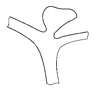
After extracting a set of points \((x,y)\) that modeled the contour of Figure 2, the parameterized was made out of the data, considering the parameter \(t\). The data was organized as shown in the Table 3.
| \(t\) | \(1\) | \(2\) | \(\cdots\) | \(39\) | \(40\) |
|---|---|---|---|---|---|
| \(x(t)\) | \(28.392\) | \(34\) | \(\cdots\) | \(43\) | \(28.392\) |
| \(y(t)\) | \(74.021\) | \(55.167\) | \(\cdots\) | \(95.417\) | \(74.021\) |
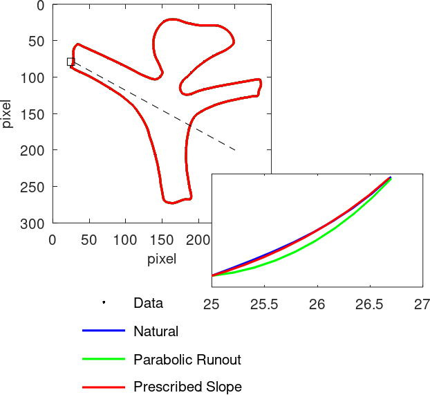
We calculated the cubical splines by the conditions (a), (b), and (c), namely: Natural, Approximation by parabola and Prescribed slope.
For the illustration of the last case, we took the values of the spline derivatives in \(x\) by:
| \(g_1^x=5.608\) | and | \(g_{40}^x=-14.608\) |
and for the derivatives of spline \(y\) considered:
| \(g_1^y=-18.854\) | and | \(g_{40}^y=-21.396\). |
It can be seen in Figure 3, in an amplification that in fact we do not have an agreement between the curves resulting from the conditions (a), (b), and (c) that were imposed on the linear system, associated with the representation of the Aneurysm geometry, for example.
Igapó lake
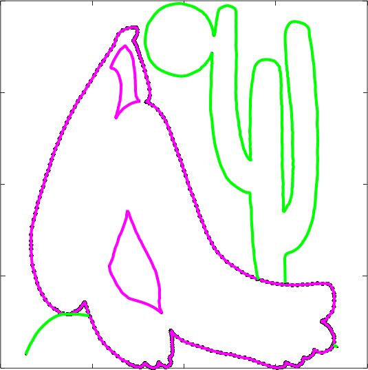
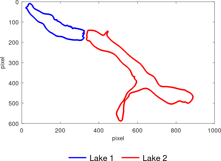
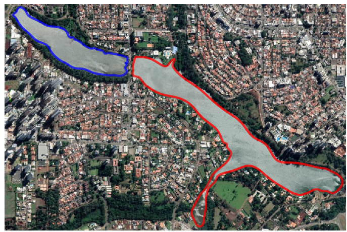
As another example, we built the splines of the edge’s Igapó lake geometry, located in Londrina Paraná, illustrated in Figure 4.
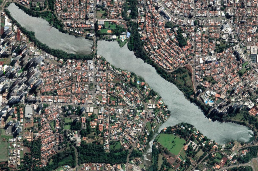
From "[Lake Igapó]", by Google .
To do that it was extracted the coordinates of the pixels contouring the lake. We tabulated and also calculated the parameterized natural cubic spline, which resulted in Figure 5. The Figure 6 shows the overlay of the splines on the image of Lake Igapó.
Considering the possibility use one of the three conditions, (a) to (c), at the system that modeled the problem, it can also to result in non-coincident curves, similar to what we showed for the Aneurysm geometry.
With what has been shown so far in the set of examples presented, observe that it is necessary some quantitative measure that expresses accuracy and supports the use of spline interpolation, submitted to some imposed condition and its extremes. With this problem, this work comes to present the modeling of a quality parameter.
Modeling a quality parameter
To qualify the computer reconstruction method of the geometry, it was modeled a parameter of quality calculated iteratively.
The proposed model is the calculate of the area between the cubic and linear splines for two consecutive intersections. After that, we inserted additional data to the initial set. So, the area between the splines is calculated again. The absolute error between those areas is calculated too. In the case of convergence satisfying a stopping criterion \(\epsilon >0\), the quality is defined. The calculate areas are an indication of the computational reconstruction’s quality. This process is shown on the flowchart presented in the Figure 7.
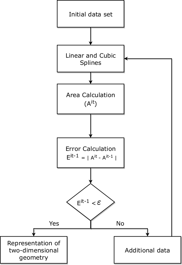
Therefore, it is necessary to define the process of calculating areas by integration and the error between them. The iterations will end the error between two consecutive areas is smaller than the pre-established stop criteria \(\epsilon >0\). The last area calculated was named quality parameter, which will indicate the fidelity of the representation.
To define the parameter, some mathematical tools are necessary, and those are mentioned below.
Mathematical tools
The quality parameter is the result of an area calculated by the integration between intersections of cubical and linear splines. The integration intervals are given by two consecutive points at which the splines intersect. By definition, we also need to know the points which are not knots, but are where the splines coincide, in other words, one point \(\xi\) such as \(SL(\xi) = SC(\xi)\). By that, is necessary to determine the real zeros of the function \((SC-SL)(x)\), where \(SC\) and \(SL\) are functions defined in equations (1) and (2).
Real zeros of the real functions
Firstly, is necessary to verify if the function \((SC-SL)(x)\), has a zero between two consecutive knots. For that, admitting the interpolators splines \(SC\) and \(SL\) of the data presented in the Table 1. According to the functions’ zero existence theorem (Ruggiero & Lopes, 1997) the following procedure was made:
considering the error \(\gamma>0\)
- -
-
this error becomes necessary to contemplate because \(x_i\) and \(x_{i+1}\) are zeros of the function \(SC-SL\). Thereby, we cannot affirm the existence of the zero according to functions’ zero existence theorem;
calculating the following product
(4)
\[ (SC-SL)(x_i+\gamma) \cdot (SC-SL)(x_{i+1}-\gamma)\]
- -
-
in case the result of equation (4) is negative, there is at least one zero between \(x_i\) and \(x_{i+1}\).
If the result of equation (4) is positive, we cannot affirm the existence of zeros.
Nonetheless, because \(SC-SL\) is a polynomial function of degree 3 and has two real zeros, \(x_i\), and \(x_{i+1}\), so the third root can only be one real number less than \(x_i\), more than \(x_{i+1}\), or that is in the interval made by the error \(\gamma\).
All these cases are not of interest to the study.
Therefore, to assert the existence of \(\xi\) it is necessary to verify the signal of the mathematical expression, equation (4). The \(\xi\) calculation will be made out by the Bisection Method deducted in Ruggiero & Lopes, 1997.
Integral between splines
Consider the function \(f\) displayed in Table 1, and the definitions of linear and cubic spline. Let \(X^1=\{x_1,x_2,...,x_m\}\) be the set of intersection points between the splines, where \(m\) is the number of nodes plus the number of intersections between them. To determine the integral difference between the splines, we need to identify:
which spline, cubic or linear, is the largest between two consecutive points of the \(X^1\) that is, if \(SL(x)>SC(x)\) or \(SL(x)
the indefinite integrals of the spline linear and cubic functions are respectively given in the forms:
(5)
\[ \int SL_k(x) dx = \dfrac{m_k}{2} \cdot x^2 + l_k \cdot x + K_1\]
\[\int SC_k(x) dx =\dfrac{a_k}{4} (x-x_k)^4 + \dfrac{b_k}{3} (x-x_k)^3 \nonumber\]
(6)
\[ + \dfrac{c_k}{2} (x-x_k)^2 +d_k x + K_2\]
with \(K_1 \in \mathbb{R}\), \(K_2 \in \mathbb{R}\) and \(k=2,\cdots,n+1\).
In this way, we can use the equations (5) and (6) to calculate the area between each spline in the intervals \([x_1,x_2],\cdots, [x_{m-1},x_{m}].\)
If \(SL \geq SC\) in \([x_{i-1},x_i]\), with \(i=2,\cdots,m\), then the area is given by
\[\begin{aligned} \int_{x_{i-1}}^{x_i} \!\!\!(SL-SC)(x) dx = \int_{x_{i-1}}^{x_i} \!\!\!\!\!SL(x) dx - \int_{x_{i-1}}^{x_i} \!\!\!\!\!SC(x) dx. \end{aligned}\]
If \(SL < SC\) in \([x_{i-1},x_i]\), with \(i=2,\cdots,m\), then calculating the area between \([x_{i-1},x_i]\), so
\[\begin{aligned} \int_{x_{i-1}}^{x_i} \!\!\!(SC-SL)(x) dx =\int_{x_{i-1}}^{x_i} \!\!\!\!\!SC(x) dx - \int_{x_{i-1}}^{x_i} \!\!\!\!\!SL(x) dx. \end{aligned}\]
We notice that \[\begin{aligned} \displaystyle\int_{x_{i-1}}^{x_i} (SC-SL)(x) dx = -\displaystyle\int_{x_{i-1}}^{x_i} (SL-SC)(x) dx. \end{aligned}\]
The area between each intersection is obtained by the equation (7), where
(7)
\[\begin{aligned} I_i = \Big|\displaystyle\int_{x_{i-1}}^{x_i} (SC-SL)(x) dx \Big| \end{aligned}\] with \(i=2,\cdots,m\).
From the mathematical tools properly defined, we can deduce a model for the quality parameter, as follows.
Quality parameter modeling
The indicator of accuracy in geometric representations modeled by spline, known as the quality parameter, is defined by:
(8)
\[ A^{it} = \sum_{i=2}^{m} I_i,\] with \(it = 1, \cdots, it_{max}\).
Notice that \(it\), equation (8), is the iterative level of the convergence process associated with the areas, and the \(it_{max}\) is the maximum number of iterations in the iterative process.
Iterative process
Inserting additional data
To insert additional data into the data set, we need to consider more points in the image. Therefore, we will look at a method for choosing the additional \(x\) values. Let \(C_0 = \left\{ x_1, x_2, \cdots, x_{n}, x_{n+1}\right\}\) be the initial set of nodes. The new set, \(C_1\), besides containing \(C_0\) has the arithmetic mean between two consecutive nodes, i.e, \[C_1 = \left\{ x_1, \dfrac{x_1+ x_2}{2}, x_2, \cdots, x_{n}, \dfrac{x_{n} + x_{n+1}}{2}, x_{n+1}\right\}.\]
Otherwise, we consider an initial set of nodes \(C_0\) with \(q_0\) points. With the proposed method, the next set \(C_1\) will have the nodes number equal to \(q_1 = q_0 + (q_0-1)\). In this way, we can define the nodes’ amount in the set \(C_p\), after \(p\) insertions of the nodes, with \(p \in \mathbb{N}\), by:
\[Q(0)=q_0, \nonumber\] and
(9)
\[ Q(p)=2\cdot Q(p-1) - 1, p\geq 1.\]
Solving this recurrence relation by expanding ([Fund_Mat_Comp_Judith - not found]), i.e. applying into equation (9) the steps \(p\), \(p-1\), \(p-2\) and so on, we get that
(10)
\[\begin{aligned} \nonumber Q(p)&=2\cdot Q(p-1) - 1 =2\cdot [2\cdot Q(p-2) - 1] - 1 \\ \nonumber &= 2^2 \cdot Q(p-2) - 2^2 + 1 \\ \nonumber &=2^2 \cdot [2\cdot Q(p-3) - 1 ] - 2^2 + 1 \\ &= 2^3 \cdot Q(p-3) - 2^3 + 1 = \cdots \end{aligned}\]
After \(k\) successive expansions, the equation (10) will have the form:
(11)
\[ Q(p) = 2^k \cdot Q(p-k) - 2^k + 1.\]
We consider the equation (11) expansion when
\(Q(p-k) = Q(0)\), i.e, \[p-k=0 \Rightarrow k=p.\]
Therefore, we get the expression
(12)
\[ \begin{aligned} Q(p) = 2^p \cdot Q(0) - 2^p + 1 = 2^p \cdot q_0 - 2^p + 1, \end{aligned}\]
which is the solution to the problem, equation (9), in closed-form.
Finally, we prove by induction that in fact the equality in equation (12) is the closed-form solution, as follows:
for \(p=1\), the equation (12) is true. In fact \(Q(1) = 2q_0 - 1\). How \(2^1 \cdot q_0 - 2^1 + 1 = 2 \cdot q_0 - 1\) so, \(Q(1)=2^1 \cdot q_0 - 2^1 + 1\).
assume that equation (12) is valid for \(p=k\). We consider the induction hypothesis given by:
(13)
\[\begin{aligned} Q(k) = 2^k \cdot q_0 - 2^k + 1. \end{aligned}\]
So, by equations (9) and (13) we have
\[\begin{aligned} Q({k+1})&= 2\cdot Q({k})-1= 2 (2^k \cdot q_0 - 2^k + 1) -1, \\ &= 2^{k+1} \cdot q_0 - 2^{k+1} + 1. \end{aligned}\]
Therefore, in fact we can calculate the number of nodes for a set \(C_p\), after the process of inserting new data, using the equality from equation (12).
Error
To check the convergence of the method, we will analyze the absolute error between the areas calculated with the nodes increases. The absolute error is given by
\[E^{it-1} = |A^{it}-A^{it-1}|,\] with \(it=2,\cdots,it_{max}\).
The process of increasing the nodes set and calculating the areas is carried out until the absolute error is less than a given stopping criterion \(\epsilon >0\). The value of the last area calculated will be the quality parameter.
Generalization to parameterized spline
To get the parameterized cubic spline, we need to apply the method proposed for the splines constructed in \((t,x(t))\) and \((t,y(t))\), separately. Therefore, we will calculate the areas for the spline in \(x\) (\(I^{x}_i\)) and in \(y\) (\(I^{y}_i\)) according to equation (7). With this, the quality parameters for these processes are defined by:
\[\begin{aligned} A_x^{it} = \sum_{i=2}^{m} I^{x}_i, A_y^{it} = \sum_{i=2}^{m} I^{y}_i, \end{aligned}\] with \(it = 1, \cdots, it_{max}\).
The convergence process of the error is studied separately for each spline. However, the iterations will only end when the error of both interpolations is less than the stopping criterion.
Results
In the Images interpolation section, we presented two geometries-2D, this time we will analyze the qualities of these representations by means of the parameter defined in this work.
Aneurysm
We calculated the quality parameter, represented by spline, of the image displayed in Figure 2. Starting from a set of \(C_0\) nodes with 40 tabulated points, and considering the stopping criterion for the error equal to \(\epsilon=0.1\), the interpolation found, for the three conditions – natural, approximation by parabola, and prescribed slope – is displayed in Figure 3.
| (a) | (b) | (c) |
 |  | 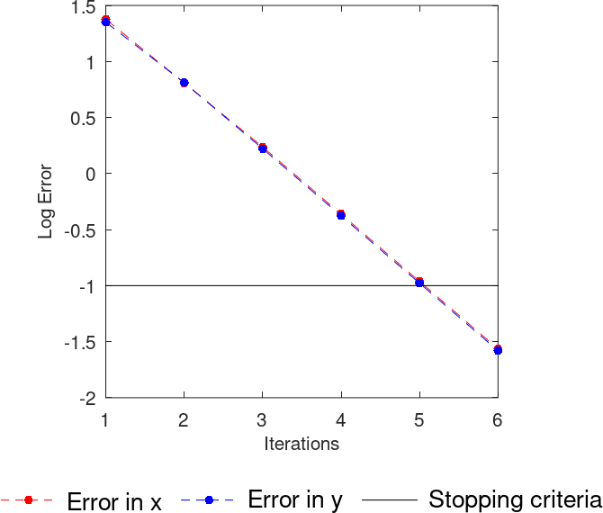 |
The areas between splines, from successive insertions calculated by our code, resulted at the values displayed in the Table 4. Based on these quantitative values, which can be seen in Figure 8, it is possible to affirm that there is indeed a convergence process for any of the three conditions. Clearly – with successive iterations – there is a quantitative reduction in the error, where the \(y\) axis represents the values of the logarithm of the errors at each iteration.
| Natural | Approximation | Prescribed | ||||
| by parabola | slope | |||||
| \(it\) | \(A_x^{it}\) | \(A_y^{it}\) | \(A_x^{it}\) | \(A_y^{it}\) | \(A_x^{it}\) | \(A_y^{it}\) |
| 1 | 33.45 | 31.98 | 32.58 | 31.12 | 32.73 | 31.04 |
| 2 | 8.819 | 8.774 | 8.744 | 8.693 | 8.748 | 8.682 |
| 3 | 2.320 | 2.241 | 2.306 | 2.225 | 2.306 | 2.222 |
| 4 | 0.582 | 0.563 | 0.579 | 0.559 | 0.579 | 0.558 |
| 5 | 0.146 | 0.141 | 0.145 | 0.140 | 0.145 | 0.139 |
| 6 | 0.036 | 0.035 | 0.036 | 0.035 | 0.036 | 0.034 |
| 7 | 0.009 | 0.008 | 0.009 | 0.008 | 0.009 | 0.008 |
Therefore, after seven iterations according to the previously defined stopping criterion, the iterative process ended and the quality parameters calculated under the different conditions for the image displayed in Figure 2, are displayed in Table 5.
| parameter in \(x\) | parameter in \(y\) | |
|---|---|---|
| Natural | 0.0091 | 0.0088 |
| Approximation | 0.009 | 0.0087 |
| by parabola | ||
| Prescribed | 0.0090 | 0.0087 |
| slope |
Note that the values found are very close, which is equivalent to saying that any of the conditions are sufficient to express the image of the aneurysm, i.e., the computer representation preserves the detail of the edge of the image. In other words, regardless of the cubic slope associated with the natural, parabola approximation, or prescribed slope, achieving the required level of detail took seven iterations. Additionally, we started with a set of \(40\) points. In the last set, we reached a total of \(2623\) nodes.
Igapó lake
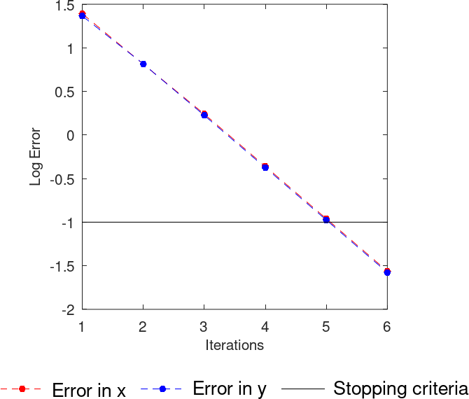
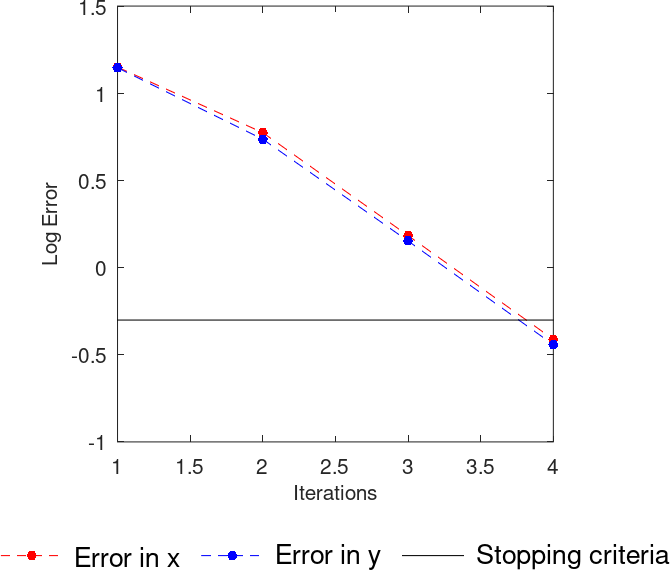
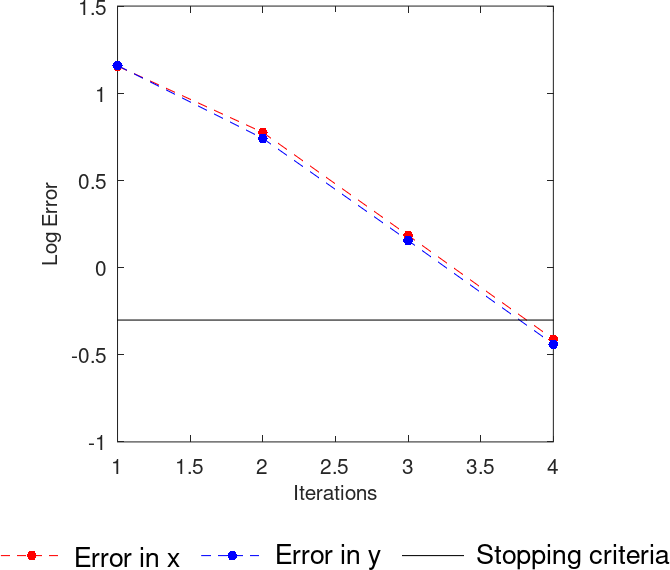
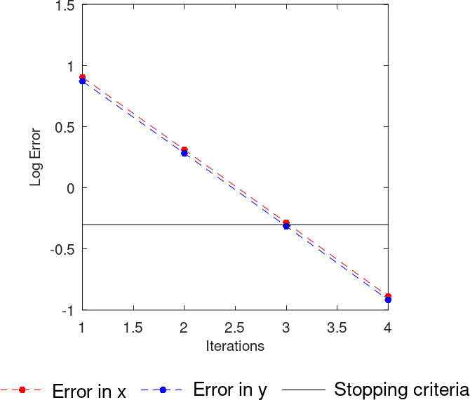
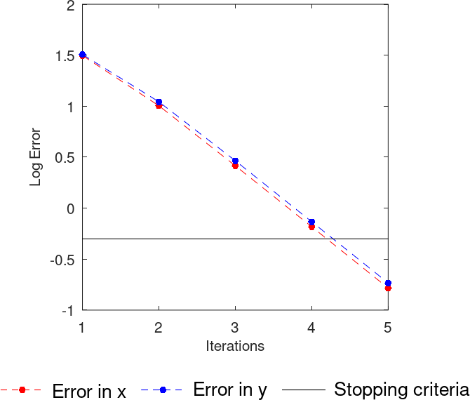
To represent the Igapó lake, see Figure 5, it was necessary to construct two splines. The stopping criterion chosen was \(\epsilon = 0.5\), and the convergence process over the two interpolations is shown in Figure 9 for lake 1, and in Figure 10 for lake 2. The quality parameters are shown in Table 6.
| (a) | (b) | (c) |
 |  |  |
| (a) | (b) | (c) |
 | 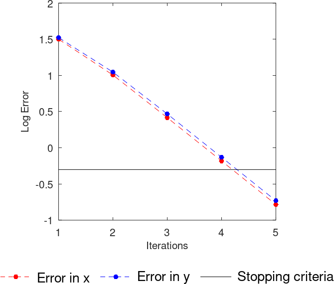 | 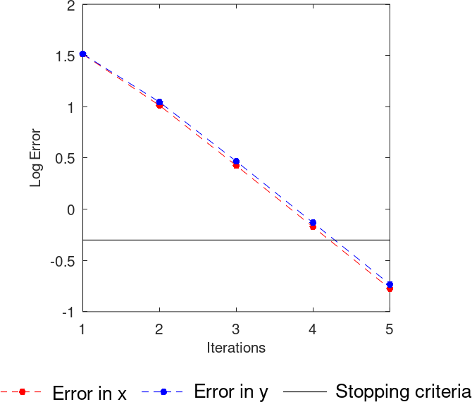 |
| parameter in \(x\) | parameter in \(y\) | ||||
| lake 1 | lake 2 | lake 1 | Lake 2 | ||
| Natural | 0.1294 | 0.0548 | 0.1205 | 0.0615 | |
| Approximation | 0.1298 | 0.0549 | 0.1213 | 0.0619 | |
| by parabola | |||||
| Prescribed | 0.1296 | 0.0560 | 0.1205 | 0.0617 | |
| slope | |||||
Note that the values found for Igapó lakes are also very close. Whichever condition is used, it is sufficient to reproduce the design of lakes 1 and 2. In this example, we needed 5 iterations for lake 1 and 6 iterations for lake 2, which allowed us to achieve a good similarity between the image and its version reproduced by splines. We emphasize that in lake 1, we started with a set of \(64\) points, and in the last set, we totaled \(2017\) nodes, whereas in lake 2, we started with \(71\) nodes, and in the last set we got \(4481\) nodes.
Conclusions
In this work, we have proposed a methodology for reconstructing the contours of a two-dimensional geometry using splines. We present general concepts and definitions for interpolating tabulated data sets. Specifically, we parameterized curves that could not be described by functions and obtained them by interpolating the data.
It is not common to have quantitative methods in commercial computer codes that monitor and qualify the fidelity of the construction of an image. However, we have defined and modeled a quality parameter for the interpolation technique discussed in this paper that could be incorporated into such codes. This model compares the proximity between cubic and linear splines by calculating the areas between these splines. In addition, the algorithm in our model increases the data set, enriching the version of the image in detail using a data insertion stop criterion.
Finally, we can see in the examples presented that the choice between the conditions of natural, approximation by parabolas, and prescribed slope is not a determining factor in the representativeness of an image by splines. However, the amount of data is a determining factor in qualification. In view of this, the way in which the new insertions are performed must guarantee accuracy and qualified imaging, which was the purpose of this work. This observation indicates that more mathematical studies are needed on how to perform data insertion optimally. Of course the images with a large amount of data can slow down the convergence process, causing prohibitive computational costs. Therefore we will move in this direction by expanding this discussion in the numerical context in a future article.
Author contributions
E.R. Cirilo participated in the: conceptualization, formal analysis, supervision, and preparation of the original manuscript. B.R. Martins Figliaggi participated in the: build of the algorithm, validation and visualization, and writing of the draft. P.L. Natti participated in the: revision and edition of the manuscript.
Conflicts of interest
The authors declare no conflict of interest.
Acknowledgments
Our thanks to the Mathematics’ PET team of the Londrina State University, and the Higher Education Secretariat of the Education Ministry, and to the Education Development National Fund, by the grant that financed this project.
References
Cirilo, E. R., & de Bortoli, Á.L. (2006). Cubic Splines for Trachea and Bronchial Tubes Grid Generation. Semina: Ciências Exatas e Tecnológicas, 27(2), 147–155. https://doi.org/10.5433/1679-0375.2006v27n2p147
Eaton, J.W., Bateman, D., Hauberg, S., & Wehbring, R. (2022). GNU Octave version 7.1.0 manual: A high-level interactive language for numerical computations. https://www.gnu.org/software/octave/doc/v7.1.0/
Enjilela, E., Lee, T.-Y., Wisenberg, G., Teefy, P.J., Bagur, R., Islam, A., Hsieh, J., & So, A. (2019). Cubic-Spline Interpolation for Sparse-View CT Image Reconstruction With Filtered Backprojection in Dynamic Myocardial Perfusion Imaging. Tomography, 5, 300–307. https://doi.org/10.18383/j.tom.2019.00013
Figliaggi, B.R.M., & Cirilo, E.R. (2021). Spline: uma ferramenta matemática. In V.P. Matias, G.S.P. Menani, A. A. Campos, & P. A. L., Fº. (Eds), Coleção de Pesquisas do Petmat (Vol.2, pp. 164-203). Universidade Estadual de Londrina. https://www.uel.br/programas/petmat/pages/arquivos/colecao/2021_v_online_v2.pdf
Gersting, J. (2014). Mathematical Structures for Computer Science. Macmillan Learning. https://books.google.com.br/books?id=unyTnQEACAAJ
Google. (2022). [Igapo Lake Londrina, Brasil]. Retrieved March, 2022. https://tinyurl.com/ylryj9jy
Habermann, C., & Kindermann, F. (2007). Multidimensional Spline Interpolation: Theory and Applications. Computational Economics, 30, 153–169. https://doi.org/https://doi.org/10.1007/s10614-007-9092-4
Pixel. (2023). In Wikipedia: The Free Encyclopedia. https://en.wikipedia.org/wiki/Pixel
Rohatgi, A. (2020). Webplotdigitizer: Version 4.4.
Ruggiero, M.A.G., & Lopes, V.L.R. (1997). Cálculo numérico: Aspectos teóricos e computacionais. Editora Pearson.
Saita, T.M., Natti, P.L., Cirilo, E.R., Romeiro, N.M.L., Candezano, M.A.C., Acuña, R.B., & Moreno, L.C.G. (2017). Simulação numérica da dinâmica de coliformes fecais no lago Luruaco, Colômbia. Trends in Computational and Applied Mathematics, 18, 435–447. https://doi.org/https://doi.org/10.5540/tema.2017.018.03.435
Zachariadis, O., Teatini, A., Satpute, N., Gómez-Luna, J., Mutlu, O., Elle, O.J., & Olivares, J. (2020). Accelerating B-spline interpolation on GPUs: Application to medical image registration. Computer Methods and Programs in Biomedicine, 193, 105431. https://doi.org/https://doi.org/10.1016/j.cmpb.2020.105431