
Reactive-Advective-Diffusive Models for the Growth of Gliomas Treated with Radiotherapy
Machado, B. S.; Alvarez, G. B.; Lobão, D. C.
DOI 10.5433/1679-0375.2023.v44.47321
Citation Semin., Ciênc. Exatas Tecnol. 2023, v. 44: e47321
Abstract:
Gliomas are malignant brain tumors responsible for 50% of primary human brain cancer cases. They have a combination of rapid growth and invasiveness, and high fatality rates with a median survival time of one year. Mathematical models that describe its growth have helped to improve treatment. In this paper, a combined model formed by terms of two other models known in the literature is analyzed. The combined model is a Reactive-Advective-Diffusive partial differential equation, which is solved by combining the finite difference method, the Crank-Nicolson method and the extitupwind method. Logistic growth is used for cell proliferation ensuring a saturation threshold for glioma growth, which is crucial to properly estimate patient survival time. The well-known linear-quadratic radiobiological model is used to describe cell death due to radiotherapy treatment. Two initial conditions are compared in the simulations, indicating the need for further studies to have a model as close as possible to reality. Simulation results are shown for four scenarios: no radiotherapy, application of a single dose, and two dose fractionation schemes.
Keywords: tumor growth, finite differences, glioblastoma, radiotherapy, mathematical models
Introduction
Gliomas are diffuse and highly invasive brain tumors that represent about 50% of all primary brain tumors (Kristin R. Swanson et al., 2003), and 23% of this percentage are the most malignant form: Glioblastoma Multiforme (Stein et al., 2007). The diagnosis of this disease depends on several factors, including the histological type and degree of malignancy, the age, and the functional neurological level of the patient. Glioma cells, in addition to rapidly proliferating, can migrate (Kristin R. Swanson et al., 2003). This invasiveness differentiates it from solid tumors, making it difficult to define the classic growth rate as the doubling of volume over time. Furthermore, the boundary between tumor and healthy tissue is not sharpened, and the number of malignant cells in healthy tissue is still undetermined. Median survival time ranges from 6 months to 1 year for patients with untreated high-grade glioma (Silva et al., 2016; Stein et al., 2007). Even slow-growing gliomas can rarely be cured by radical surgical resection. In general, they are not encapsulated, and even apparently encapsulated ones such as ependymomas are not treatable by simple surgical resection (Shuman et al., 1975). Furthermore, gliomas can show very high proliferation rates, with doubling times ranging up to 1 week in vivo.
The processes that govern glioma invasion and aggressiveness are poorly understood. Also, conventional therapies (surgery, radiotherapy and/or chemotherapy) have offered little improvement in patient lifespan. All of this has motivated the emergence of mathematical models to help with treatment planning (Silva et al., 2016). Two mathematical models that describe the growth of gliomas were proposed in Leder et al., 2014, Rockne et al., 2009 and Kristin R. Swanson et al., 2003. Both models were analyzed in Barbosa et al., 2019, Silva et al., 2016 and Souza et al., 2015, and new approaches based on time series were suggested in Jesus et al., 2014 and Silva et al., 2021.
However, our previous analyses do not include the non-linear term that saturates cell growth for the model proposed in Rockne et al., 2009. Here, the non-linear term and a new term suggested in Stein et al., 2007 are included. Thus, a combined model based on Rockne et al., 2009 and Stein et al., 2007 is analyzed. This model is of the Reactive-Advective-Diffusive type for cell proliferation, invasion, and migration (Stein et al., 2007), and contains the term that describes the effect of radiotherapy (Rockne et al., 2009).
The main objective of this work is to apply the finite difference method to solve the combined model, and to analyze the response of this glioma model to radiotherapy with different dose fractional schemes. That is, there are no results for the combined model in the literature. This is one of the main novelties of our work. The model described in Rockne et al., 2009 does not consider an advective term for invasive cells. The model described in Stein et al., 2007 does not consider the radiotherapy response term. As far as the authors are aware, this is the first time that all these terms are combined in a single framework. Furthermore, an initial condition different from the one proposed in Rockne et al., 2009 is explored. The shape of the two considered initial conditions is very similar. The main difference between these two initial conditions lies in the mathematical properties of the functions, since one initial condition is continuously differentiable and the other is a continuous function with the first derivative discontinuous at three points. The initial condition is an initial picture of the tumor, which must evolve over time according to the characteristics of the mathematical model. In general, this picture is constructed based on non-invasive images generated by various diagnostic techniques, such as computed tomography and magnetic resonance imaging. Even with today’s advanced technology, there are great uncertainties in defining the boundary between tumor and healthy tissue. For this reason, it is common to use a safety margin in radiotherapy. Our study shows that two very similar initial pictures develop over time with significant differences. This is another contribution of this work, as it shows that two very similar initial conditions can produce very different results.
The rest of the paper is organized as follows. In the next section, the combined model is presented together with the two initial conditions studied. The Methodology section describes the combination of finite difference, Crank-Nicolson and upwind methods used to solve the models. Simulation results are shown for four scenarios in the Results and discussion section. Our final comments are presented in the Conclusions.
Combined model of tumor growth
Most continuous models consist of differential equations that describe the dynamics of cancer cells based on rates of change of quantities of interest. The combined model analyzed here is composed of some terms from two continuous models presented in Stein et al., 2007 and Rockne et al., 2009 that simulate glioma as a spheroid tumor. Both models consider a reactive term to describe cell proliferation and a diffusive term to describe cell migration, as shown in equation (1):
(1)
\[ \frac{\partial u(r,t)}{\partial t} = \underbrace{D\nabla^2u}_{{\tiny Diffusion}} + \underbrace{gu\left(1 - \frac{u}{u_{max}}\right)}_{{\tiny Proliferation}},\]
where \(u(r, t)\) is the concentration of tumor cells \((cells/cm^3)\) in the spatial position \(r=(x,y,z)\) at the instant of time \(t\), \(D\) is the diffusion coefficient with dimensions \((cm ^2/day)\), \(g\) is the proliferation rate in \((1/day)\), and \(u_{max}\) is the maximum concentration of tumor cells in \((cells/cm^3)\). Cell proliferation is modeled assuming logistic growth, where the non-linear term guarantees saturation of cell growth. That is, the concentration of tumor cells will never be greater than \(u_{max}\) or the tumor stops growing when \(u(r, t)=u_{max}\). The maximum concentration is estimated as \(u_{max} = 4.2\) \(10^8\) \(cells/cm^3\) assuming that the volume of a typical cell is \(1200\) \(\mu m^3\) and that half the volume of the spheroid is composed of tumor cells (Stein et al., 2007).
Experimental data show that the model, equation (1), fails for tumors with a radius smaller than 1 \(mm^3\) (Stein et al., 2007). So, in Stein et al., 2007 it is suggested that small tumors are formed by two cell populations that present different proliferative and dispersive behaviors: a central core and an invasive border. Core cells proliferate rapidly and move slowly. Invasive border cells proliferate slowly and move quickly. Thus, in addition to the two terms in the equation (1), an advective term is added to the dispersion of invasive cells
(2)
\[ \frac{\partial u(r,t)}{\partial t} = \underbrace{D\nabla^2u}_{{\tiny Diffusion}} + \underbrace{gu\left(1 - \frac{u}{u_{max}}\right)}_{{\tiny Proliferation}} -\underbrace{ v \cdot \nabla u}_{{\tiny Advection}},\]
where \(v\) is the average velocity with which the invasive cells move away from the core (Stein et al., 2007). Furthermore, in Stein et al., 2007 a source term of the type Dirac delta function is introduced to model the growth of the core. However, this source term will not be considered in the combined model. This is because this term is important to describe the growth of small tumors with a radius between 0.1 \(mm\) and 0.5 \(mm\), and in all our simulations, tumors with an initial radius of 1.41 \(cm\) were considered.
On the other hand, the model, equation (2), does not consider cell death due to radiotherapy treatment.
As presented in Rockne et al., 2009, radiotherapy introduces a new term to the equation (2), resulting in:
(3)
\[ \frac{\partial u}{\partial t} = D\nabla^2u + gu\left(1 - \frac{u}{u_{max}}\right) - v \cdot \nabla u - A(d(r,t))u,\]
where
(4)
\[ A(d(r,t)) = \begin{cases} 0 & t \notin \text{therapy}\\ 1 - S(d(r,t)) & t \in \text{therapy} \end{cases},\]
and \(S(d(r,t))\) is the probability of cell survival after applying the dose per fraction \(d(r,t)\).
Considering the Linear-Quadratic (LQ) radiobiological model (Eric, 2000; Michael C. Joiner & Albert J. van der Kogel, 2009), the fraction of surviving cells \(S(D)\) after radiotherapy with a single total dose \(D\) in Gray units \((Gy)\) is
(5)
\[ S(D) = e^{\left(-\alpha D -\beta D^{2}\right)},\]
where \(\alpha\) and \(\beta\) are cell line-specific parameters determined by cell survival experiments. It is frequent to assume constant \(\alpha/\beta\), and in the case of gliomas \(\alpha/\beta = 10\). In radiation oncology, dose fractionation is preferable to a single dose, as there is experimental evidence showing therapeutic gain. In addition, fractionation seeks to reduce the toxic effect of radiation on healthy tissue. Thus, a total dose \(D=nd\) is divided into \(n\) equal doses \(d=d(r,t)\) which are applied maintaining the same time interval between fractions. Therefore, the probability of cell survival after delivering the dose per fraction \(d\) is
(6)
\[ S(d(r,t)) = e^{\left(-\alpha d -\beta d^{2}\right)}.\]
The partial differential equation (PDE), given in equation (3), is of the reaction-advection-diffusion (RAD) type, and represents the combined model that will be analyzed here. This equation needs an initial condition \(u(r,0) = u_{0}(r)\) and boundary conditions for the model to be mathematically well-posed. As presented in Rockne et al., 2009, gliomas rarely metastasize which justifies a Neumann-type boundary condition \(\hat{n} \cdot \nabla u = 0\) for all points on the brain border, where \(\hat{n}\) denotes the unit normal vector exiting the boundary. This boundary condition means that there are no cancer cells coming out of the brain.
One-dimensional dimensionless model
For simplicity, our analysis will be carried out only for the one-dimensional case, where the spatial domain is defined by \(x \in [0,L]\), and \(L=20\) \(cm\) is the length of the domain. In the one-dimensional case the combined model is described as
(7)
\[ \dfrac{\partial u}{\partial t} = D \dfrac{\partial^2 u}{\partial x^2} - v \dfrac{\partial u}{\partial x} + gu\left(1 -\dfrac{u}{u_{max}}\right) - A(d(x,t))u,\]
with initial and boundary conditions given by
(8)
\[ u_1(x,0) = u_0 e^{-100(x/L)^{2}},\]
(9)
\[ \dfrac{\partial u}{\partial x} = 0 \text{ if } x=0 \text{ or } x=L,\]
\(u_0\) is the initial maximum concentration of tumor cells whose value is \(u_0 =\) 8000 \(cells/cm^3\).
The initial condition, equation (8), is introduced in Rockne et al., 2009, which is a continuously differentiable function. Our analysis includes a new initial condition defined as
(10)
\[ u_2(x,0) = \begin{cases} U_{0} & \forall x \in ~[0,x_{m}]\\ m_1(x - x_{m}) + U_{0} & \forall x \in~ ]x_{m},x_{l}] \\ m_2(x - x_{l}) + U_{thr} & \forall x \in ~]x_{l},x_{z}] \\ 0 & \forall x \in~ ]x_{z},L] \end{cases},\]
where \(U_{0} = u_0\), \(U_{thr} = 0.6126 U_{0}\) is the detectable margin, \(U_{z} = 0\), \(m_1=\dfrac{U_{0} - U_{thr}}{x_{m} - x_{l}}\), \(m_2=\dfrac{U_{thr} - U_{z}}{x_{l} - x_{z}}\), \(x_{m} = 0.6\) \(cm\), \(x_{l} = 1.41\) \(cm\) and \(x_{z} = 2\) \(cm\). This new initial condition is a continuous function with the first derivative discontinuous at three points: \(x_{m}\), \(x_{l}\) and \(x_{z}\).
In order to construct a computational code that numerically solves the problem described above, it is convenient to write the equations in dimensionless form. In this paper, we follow the same dimensionless performed in Rockne et al., 2009 and Junior, 2014. Thus, the combined model is written in its dimensionless form by introducing the dimensionless variables \(\bar{x} = x/L\), \(\bar{t} = tg\), \(\bar{u} = u/u_{max}\). In this way, \(\bar{x} \in [0, 1]\) and \(\bar{t} \in [0, gt_f]\) being \(t_f\) the final time. After some algebraic manipulations the equation (7) is transformed as
(11)
\[ \dfrac{\partial \bar{u}}{\partial t} = D^{*} \dfrac{\partial^2 \bar{u}}{\partial x^2} - v^{*} \dfrac{\partial \bar{u}}{\partial x} + \bar{u} \big(A^{*}(d(\bar{x},\bar{t}))-\bar{u} \big),\]
where \(D^{*} = \dfrac{D}{gL^2}\), \(v^{*} = \dfrac{v}{gL}\) and
(12)
\[ A^{*}(d(\bar{x},\bar{t})) = \begin{cases} 1 & \bar{t} \notin \text{therapy}\\ 1 - \dfrac{1 - S(d(\bar{x},\bar{t}))}{g} & \bar{t} \in \text{therapy} \end{cases}.\]
Methodology
The equation (11) is solved using the finite difference method, where the Crank-Nicolson method is applied for the diffusive-reactive terms with a first order direct difference for the nonlinear term, and the upwind numerical differentiation will be used for the advective term.
Crank-Nicolson method for diffusive-reactive terms
In numerical analysis, the Crank-Nicolson method is used to solve parabolic partial differential equations numerically. Using centered differences for space, and the trapezoidal rule in time, the method is second-order in space and implicit in time.
Let us first consider only the diffusive-reactive terms of the equation (11)
(13)
\[ \dfrac{\partial \bar{u}}{\partial t} = D^{*} \dfrac{\partial^2 \bar{u}}{\partial x^2} + \bar{u}\left(A^{*} -\bar{u}\right),\]
where \(A^{*}\) is determined by the equation (12).
The equation (13) is precisely the model presented in Rockne et al., 2009 for tumor growth in response to radiotherapy. This equation is of the reaction-diffusion (RD) type, and will be compared with the combined model determined by the equation (11).
Before applying the Crank-Nicolson method a linear approximation for the non-linear term \(Y(u) = u(A^{*} - u)\) is used. According to Aggarwal (1985, p. 420) one can use the implicit method of linearization in time which, instead of linearizing \(Y(u)\) in iterative space, uses a Taylor series expansion over the known time level. Thus, applying the Crank-Nicolson method according to the methodology of S., 1985 the equation (13) is approximated as \[\dfrac{U_{i}^{k+1} - U_{i}^{k}}{\Delta t} = \dfrac{D^{*}}{2\Delta x^2} \Big((U_{i + 1}^{k} - 2U_{i}^{k} + U_{i - 1}^{k}) \nonumber\]
(14)
\[ + (U_{i + 1}^{k + 1} - 2U_{i}^{k + 1} + U_{i - 1}^{k + 1})\Big) + \dfrac{1}{2} \left(Y(U_{i}^{k+1}) + Y(U_{i}^{k})\right).\]
Upwind method for advective term
The upwind scheme is a numerical discretization method for solving hyperbolic partial differential equations. Consider only the advective term of the equation (11) we get equation (15)
(15)
\[ \dfrac{\partial \bar{u}}{\partial t} = - v^{*} \dfrac{\partial \bar{u}}{\partial x}.\]
The spatial point approximation \(i-1\) is used when the velocity \(v^{*}\) has a positive sign, i.e.
\[\dfrac{U_{i}^{k+1} - U_{i}^{k}}{\Delta t} = -v^{*}\dfrac{U_{i}^{k} - U_{i-1}^{k}}{\Delta x} \nonumber\]
if \(v^{*} \ge 0\). So the solution propagates to the right of the point \(i\), where \(i-1\) is the point “upstream”.
When the velocity has a negative sign, the solution propagates to the left, i.e.
\[\dfrac{U_{i}^{k+1} - U_{i}^{k}}{\Delta t} = -v^{*}\dfrac{U_{i+1}^{k} - U_{i}^{k}}{\Delta x} \nonumber\]
if \(v^{*} < 0\). So the spatial point \(i+1\) is the “upstream” point.
A compact form of the upwind scheme can be constructed by defining two operators
(16)
\[\begin{aligned} v^{+} = \max(v^{*},0) & \text{and} & v^{-} = \min(v^{*},0). \end{aligned}\] Combining the operators defined in equation (16) we obtain a compact form for the upwind scheme, given by
(17)
\[ \dfrac{U_{i}^{k+1} - U_{i}^{k}}{\Delta t} = -v^{+}\left(\dfrac{U_{i}^{k} - U_{i-1}^{k}}{\Delta x}\right) -v^{-}\left(\dfrac{U_{i+1}^{k} - U_{i}^{k}}{\Delta x}\right).\]
By making a linear combination of the equations (14) and (17) approximations for the combined model, equation (11), we obtain
(18)
\[ \dfrac{U_{i}^{k+1} - U_{i}^{k}}{\Delta t} = \dfrac{D^{*}}{2\Delta x^2}\Big((U_{i + 1}^{k} - 2U_{i}^{k} + U_{i - 1}^{k}) \nonumber\] \[+ (U_{i + 1}^{k + 1} - 2U_{i}^{k + 1} + U_{i - 1}^{k + 1})\Big)+\dfrac{1}{2}\Big(U_{i}^{k}A^{*} + U_{i}^{k+1}A^{*} \nonumber\] \[-2U_{i}^{k}U_{i}^{k+1}\Big) -\dfrac{v^{+}}{\Delta x}\left(U_{i}^{k} - U_{i-1}^{k}\right) -\dfrac{v^{-}}{\Delta x}\left(U_{i+1}^{k} - U_{i}^{k}\right).\]
The equation (18) can be written in the form \[-\lambda U_{i - 1}^{k + 1} + P(U_{i}^{k})U_{i}^{k+1} - \lambda U_{i + 1}^{k + 1} = S^{+} U_{i - 1}^{k}\nonumber\]
(19)
\[ + R U_{i}^{k} + S^{-} U_{i + 1}^{k},\]
where
\[\lambda = \dfrac{D^{*}\Delta t}{2\Delta x^2}, \nonumber\] \[\tau = \dfrac{\Delta t}{2},\nonumber\] \[P(U_{i}^{k}) = 1 + 2\lambda -\tau A^{*} + 2\tau U_{i}^{k},\nonumber\] \[\nu^{+} = \dfrac{v^{+}\Delta t}{\Delta x},\nonumber\] \[\nu^{-} = \dfrac{v^{-}\Delta t}{\Delta x},\nonumber\] \[R = 1 - 2\lambda + \tau A^{*} - \nu^{+} + \nu^{-},\nonumber\] \[S^{+} = \lambda + \nu^{+} \nonumber\]
and
\[S^{-}= \lambda - \nu^{-}.\nonumber\]
Boundary points
Using second-order finite difference forward in space for the first node \(\dfrac{\partial u}{\partial x} = \dfrac{-3U_i + 4U_{i+1} - U_{i+2}}{2\Delta x}\), and backward for the last node \(\dfrac{\partial u}{\partial x} = \dfrac{3U_i - 4U_{i-1} + U_{i-2}}{2\Delta x}\), the boundary condition is approximated by equation (20) for the first node and equation (21) for the last node, given by
(20)
\[ -3U_{1}^{k + 1} + 4U_{2}^{k + 1} - U_{3}^{k + 1} = 3U_{1}^{k} - 4U_{2}^{k} + U_{3}^{k},\]
(21)
\[ -3U_{M+1}^{k + 1} + 4U_{M}^{k + 1} - U_{M-1}^{k + 1} = 3U_{M+1}^{k} - 4U_{M}^{k} + U_{M-1}^{k}.\]
The vector with the unknowns at each time step is denoted by \(\mathbf{U}^{k} = \begin{bmatrix} U_{1}^{k} \ U_{2}^{k} \ U_{3}^{k} \ \cdots \ U_{M}^{k} \ U_{M+1}^{k} \end{bmatrix}^{T}\) and \(\mathbf{U}^{k+1}~=~\begin{bmatrix} U_{1}^{k+1} \ U_{2}^{k+1} \ U_{3}^{k+1} \ \cdots\ U_{M}^{k+1} \ U_{M+1}^{k+1} \end{bmatrix}^{T}\). Thus, the equations (19)-(21) form a linear system of algebraic equations for each time step that can be solved using a direct method. Knowing an approximation in the previous step \(\mathbf{U}^{k}\), the method determines \(\mathbf{U}^{k+1}\) as the solution of the linear system
(22)
\[ \mathbf{AU}^{k+1} = \mathbf{b}^{k} = \mathbf{EU}^{k},\] where \(\mathbf{A}\) and \(\mathbf{E}\) are the tridiagonal matrices
(23)
\[ \mathbf{A} = \begin{bmatrix} -3 & 4 & -1 & 0 & 0 & 0 & 0 \\ -\lambda & P(U_{2}^{k}) & -\lambda & 0 & 0 & 0 & 0 \\ 0 & -\lambda & P(U_{3}^{k}) & -\lambda & 0 & 0 & 0 \\ \vdots & \ddots & \ddots & \ddots & \ddots & \ddots & \vdots \\ 0 & 0 & 0 & -\lambda & P(U_{M-1}^{k}) & -\lambda & 0 \\ 0 & 0 & 0 & 0 & -\lambda & P(U_{M}^{k}) & -\lambda \\ 0 & 0 & 0 & 0 & 1 & -4 & 3 \end{bmatrix},\]
(24)
\[ \mathbf{E} = \begin{bmatrix} 3 & -4 & 1 & 0 & 0 & 0 & 0 \\ S^{+} & R & S^{-} & 0 & 0 & 0 & 0 \\ 0 & S^{+} & R & S^{-} & 0 & 0 & 0 \\ \vdots & \ddots & \ddots & \ddots & \ddots & \ddots & \vdots \\ 0 & 0 & 0 & S^{+} & R & S^{-} & 0 \\ 0 & 0 & 0 & 0 & S^{+} & R & S^{-} \\ 0 & 0 & 0 & 0 & -1 & 4 & -3 \end{bmatrix}.\]
In the equation (22) it should be understood that first the matrix \(\mathbf{E}\) is multiplied with the solution vector in the previous step \(\mathbf{U}^{k}\) and then it is solved the linear system. Analysis of stability and consistency of these formulations can be found in Machado, 2023.
Results and discussion
Here, results of the evolution of glioma in response to radiotherapy are presented for the RAD and RD models, equations (11) and (13), respectively. The objective is to compare the predictions of both models to evaluate how the advective term (RAD model) influences the evolution of tumor size, in addition to comparing the impact of the two initial conditions. The two models were implemented in a computational code developed using the Matlab software.
It should be noted that the RD and RAD models were normalized for better computational code performance. However, after obtaining the dimensionless numerical solution, the results were post-processed and transformed into variables with physical dimensions. We believe that this should facilitate a better understanding of the simulations carried out.
Although the spatial domain has a length \(L = 20\) \(cm\), in Figure 1 and in the section on Final tumor cell concentration we present the results up to \(x=10\) \(cm\). In this way, the difference between all plotted curves is emphasized.
Figure 1 shows the two initial conditions defined by equations (8) and (10), in addition to the initial radius of the tumor that corresponds to the hatched region.
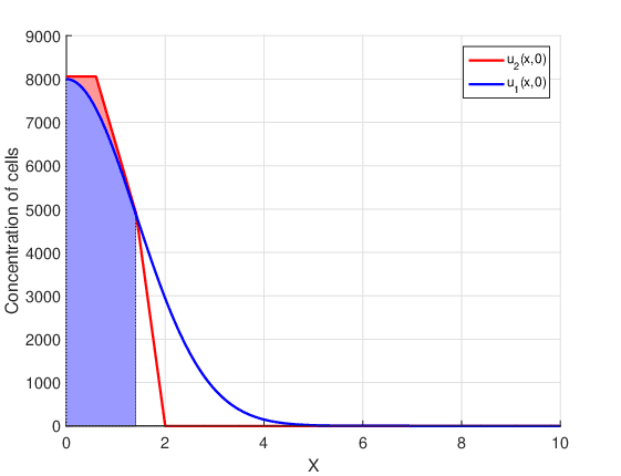
This region is determined by the detectable margin of the tumor. In other words, for concentrations smaller than the detectable margin \(U_{thr}\) the tumor radius is considered zero. At each time instant, the tumor radius is calculated as
(25)
\[ R(t^k) = \begin{cases} \max\limits_{\substack{i}} \{ x_i \} ,& \text{if } U_i^k \geq U_{thr} \\ 0,& \text{otherwise} \end{cases}.\]
The initial conditions, \(u_1(x,0)\) and \(u_2(x,0)\), have the same initial radius \(R_0=1.41\) \(cm\), but different mathematical behavior. The initial condition \(u_1(x,0)\) is introduced in Rockne et al., 2009, and is a continuous function along with all its derivatives. The initial condition \(u_2(x,0)\) is proposed for the first time in this work. Although \(u_2(x,0)\) is continuous, its derivative is discontinuous at the points that delimit the four parts. In the first part the concentration of cancer cells is a constant, in the second and third part the concentration is described by straight lines with different slopes, and in the fourth part there are no cancer cells. This last part establishes a big difference between the two initial conditions, since \(u_1(x,0) \neq 0\) for all points in the domain. That is, the initial condition \(u_1(x,0)\) assumes that there are cancer cells throughout the brain, even if at points far from the center of the tumor they are present in very small amounts.
The results of the glioma evolution simulations that the two models predict will be separated into three groups. First, concentrations at the final time point (\(t_f=80\) days) are compared. In the second group, tumor radius are compared at each instant of time. In the third group, the temporal evolution of the maximum concentrations is
presented.
Parameter values and dose fractionation
The simulations are based on the results described in Rockne et al., 2009 and Silva et al., 2016, as they allow comparisons to be made to validate the developed code. The following parameters were used as input data: initial radius \(R_0 = 1.41\) \(cm\), constant diffusion coefficient \(D = 3.9\) \(10^{-5}\) \(cm^2/day\), proliferation rate \(g = 0.0453\) \(day^{-1}\), saturation limit for cell concentration \(u_{max} = 4.2\) \(10^{8}\) \(cells/cm^3\), average velocity of invasive cells moving away from the core \(v = 0.01\) \(cm/days\), and the radiobiological model parameters \(\alpha = 0.0305\) \(Gy^{-1}\) and \(\alpha/\beta = 10\) \(Gy\).
In the treatment schemes detailed in Table 1, it was considered that all doses were applied daily at 8:00 am, and that on Saturday only a booster dose was applied depending on the fractionation scheme. On Sundays there was never a dose application. Other fractionation schemes were studied in Machado, 2023.
According to Rockne et al., 2009 (2008), days in therapy (DIT) is defined to be the duration of the therapy regimen, whereas days of treatment (DOT) is defined to be the number of days in which XRT was actually administered.
| Fractionation schemes | |
|---|---|
| DOT \(=\) 0 day | There is no treatment |
| DOT \(=\) 1 day | Dose of 60 Gy given on a single day and 4.2 Gy booster delivered the next day |
| DOT \(=\) 5 days | Dose of 12.2 Gy given each day, and 3.2 Gy booster given on day six |
| DOT \(=\) 35 days (7 weeks of treatment) | Daily dose of 1.8 Gy given during the first five days of each week, and without a booster dose |
Final goncentration of glioma cells
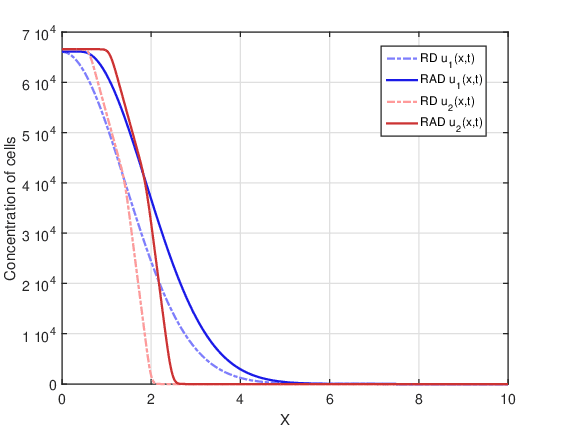
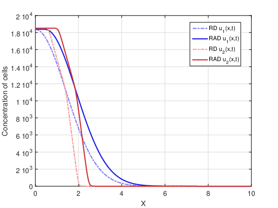
DOT \(= 0\) day:
In this case there is no therapy. Figure 2 shows tumor cell concentration as a function of \(x\) predicted by RAD and RD models for \(t_f=80\) days and the two initial conditions \(u_1(x,0)\) and \(u_2(x,0)\). It is notable that, for both initial conditions, the curve of the RAD model is wider than the prediction of the RD model. This was to be expected because the RAD model is more dispersive due to the advection term, which contributes to a greater tumor expansion compared to the RD model. It should be noted that the discontinuity points for the initial condition \(u_2(x,0)\) disappear after 80 days for both models, since these discontinuities are smoothed by the diffusion term present in both models.
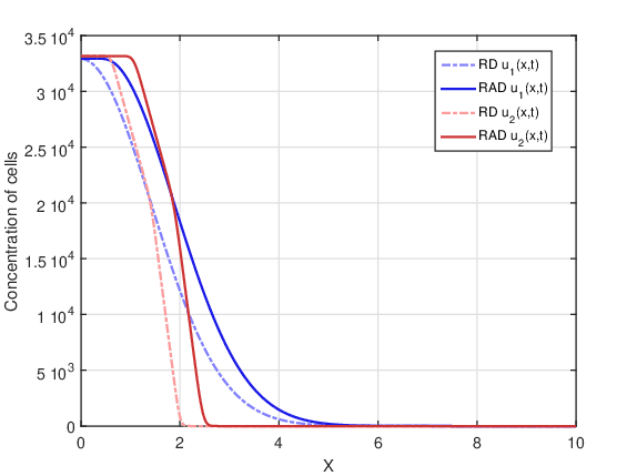
DOT\(=1\) day:
In this case, a single dose is applied. Figure 3 shows tumor cell concentration as a function of \(x\) predicted by RAD and RD models for \(t_f=80\) days and the two initial conditions \(u_1(x,0)\) and \(u_2(x,0)\). Comparing Figures 2 and 3 a decrease in concentration is observed for both models, since there was cell death due to radiotherapy. On the other hand, the shape of the curves remained similar in both figures.
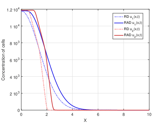
DOT\(=5\) days:
In this case, there was fractionation of the dose. Figure 4 shows tumor cell concentration as a function of \(x\) predicted by RAD and RD models for \(t_f=80\) days and the two initial conditions \(u_1(x,0)\) and \(u_2(x,0)\). Comparing Figures 3 and 4 it is possible to observe a drastic decrease in cell concentration for both models, since the fractionation of the dose is more therapeutically efficient than the treatment with a single dose. Among all fractionations, specifically this fractionation proved to be the most advantageous. In addition, the shape of the curves remained similar in Figures 2-4.
DOT \(=35\) days:
In this case, there was a larger fractionation of the dose. Figure 5 shows tumor cell concentration as a function of \(x\) predicted by RAD and RD models for \(t_f=80\) days and the two initial conditions \(u_1(x,0)\) and \(u_2(x,0)\). It is observed that this fractionation presents a lower cell concentration for both models than the single dose treatment, but a higher cell concentration than the DOT \(=5\) days fractionation. Again, the shape of the curves remained similar in Figures 2-5.
Tumor radius evolution
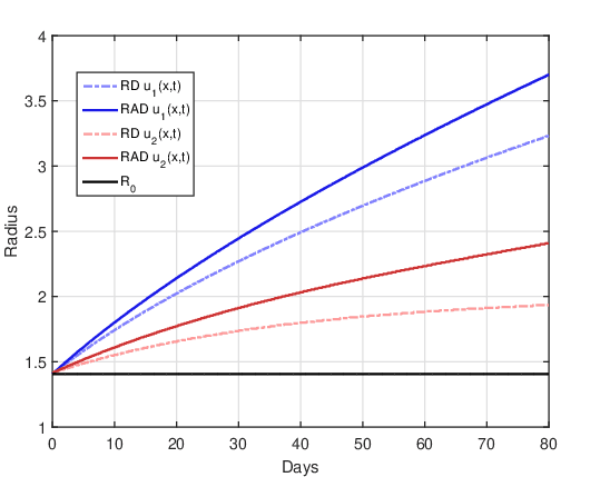
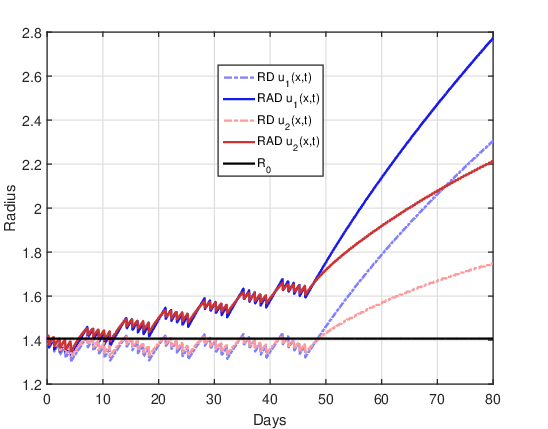
DOT \(=0\) day:
Figure 6 shows the evolution of the tumor radius over the days for the RAD and RD models and the two initial conditions. The straight line \(R(t) = R_0\) represents the initial tumor radius, which makes it easier to identify the time instants in which the tumor size is larger or smaller than the tumor before treatment. As there is no treatment, the tumor grows freely over time, since the influence of the non-linear term that saturates cell proliferation is still not significant for 80 days (\(u(x,t) << u_{max}\) \(\forall t \leq 80\)). It can also be confirmed that the tumor radius in the RAD model is notably larger than in the RD model for the two initial conditions, showing that the advective term significantly influenced tumor growth.
DOT \(=1\) day:
Figure 7 shows the evolution of the tumor radius over the days for the RAD and RD models and the two initial conditions. The single dose together with the booster dose causes the tumor radius to decrease to close to zero for a few days, and then, close to the ninth day, it grows again.
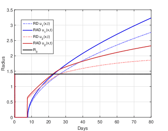
Upon resumption of tumor growth, the shape of the tumor radius curve is remarkably different for the two initial conditions. For the initial condition \(u_1(x,0)\), the growth curve of the RAD and RD models has a similar shape, where the radius estimated by the RAD model is greater than that of the RD model. The radius estimated by the RD model is similar to that presented by Rockne et al., 2009, and this can be considered a validation of our computational codes. For the initial condition \(u_2(x,0)\) in both models, it is possible to observe two significant changes in the slope of the curve after the treatment period that may possibly be related to the initial tumor radius \(R_0\). After the recession period, there is a very marked resumption in tumor growth, and when the radius exceeds the initial radius the growth rate changes again. For the RD model the moment of the second “change” in the growth rate is at the instant \(t \approx 27\) at which \(R(t) = R_0\). For the RAD model, the moment of the second “change” is shifted to a previous instant \(t \approx 25\) in which \(R(t)~>~R_0\).
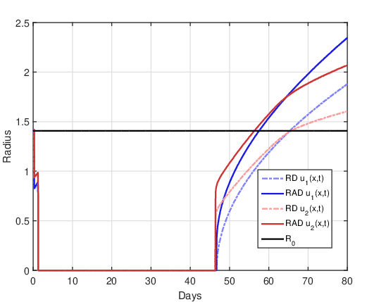
DOT \(=5\) days:
Figure 8 shows the evolution of the tumor radius over the days for the RAD and RD models and the two initial conditions. This is the most advantageous case of dose fractionation, since it presents a longer period of time (approximately 47 days) for which the tumor radius remains close to zero. After this period of time, the tumor grows again, but with significant differences between the RAD and RD models for the two initial conditions. Similar to the DOT\(=\)1 day case, the growth in the RAD and RD models has a similar shape for the initial condition \(u_1(x,0)\). Again, for the initial condition \(u_2(x,0)\) in both models there are two significant changes in the growth rate after the recession period. For the RD model the moment of the second “change” in the growth rate is at the instant \(t \approx 65\) at which \(R(t) = R_0\). For the RAD model, the moment of the second “change” is shifted to a previous instant \(t \approx 63\) in which \(R(t) > R_0\). On the other hand, comparing Figures 7 and 8 it is clear that, for both models and the two initial conditions, dose fractionation is more therapeutically efficient than treatment with a single dose.
DOT\(=35\) days:
Figure 9 shows the evolution of the tumor radius over the days for the RAD and RD models and the two initial conditions. In all curves, oscillations in the tumor radius are evident throughout the duration of radiotherapy, which are a consequence of the application of the fraction of the dose per day. For this dose fractionation scheme, there is no period of tumor recession, that is, the tumor radius is never close to zero. For both initial conditions, the impact of the advective term on tumor evolution throughout the treatment application period is evident, since the tumor radius in the RD model remains close to the initial radius while in the RAD model it grows above the initial radius. After the end of treatment, the tumor seems to grow with similar shape for both initial conditions. For the initial condition \(u_2(x,0)\), the two points of significant changes in the growth rate were not observed after the end of the treatment, unlike what was observed in the cases DOT \(=~1\) day and DOT \(= 5\) days.
On the other hand, the following observation was verified for all fractionation schemes. The RAD model solutions for the initial condition \(u_1(x,0)\) and \(u_2(x,0)\) can have several intercept points. The number of these intercepts seems to depend on the fractionation scheme, that is, it seems to be related to the number of fractions \(n\) and the value of the dose per fraction \(d\). This demonstrates that the temporal evolution of the tumor radius can switch to the RAD model when all parameters are fixed and only the initial condition is varied.
Furthermore, the difference between the tumor radius predicted by both initial conditions can be significant, especially in the region close to the last intercept. However, for all fractionation schemes, it is verified that after the last intercept between these solutions, the tumor radius predicted by the initial condition \(u_2(x,0)\) is always significantly smaller than that predicted by \(u_1(x,0)\). This same finding is also valid for the RD model, indicating that the initial condition is a crucial element in building a mathematical model as close as possible to reality.
Maximum cell concentration
Figures 10 and 11 show the evolution of the maximum cell concentration over the days for the RAD and RD models and the two initial conditions. Unlike what was observed for the final cell concentration and tumor radius, the maximum cell concentration for both models is the same. This was expected because the advective term contributes to faster tumor growth, but this term does not create or destroy cells. It is just a transport term that contributes to the dispersion of cells along with the diffusion term. The reactive term is solely responsible for cell proliferation or death.
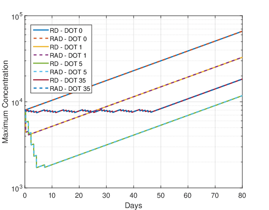
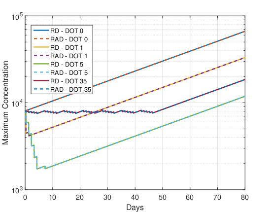
DOT \(=0\) day:
As there is no therapy, the growth of maximum cell concentration on the logarithmic scale is almost linear in Figures 10 and 11. Furthermore, the differences between the initial conditions \(u_1\) and \(u_2\) are negligible, so that the maximum concentration of both models are the same.
DOT \(=1\) day:
For this fractionation scheme a marked decrease in the maximum cell concentration can be observed during the single dose administration and a smaller decrease during the booster. After the end of the treatment application (region of the graph where there is a negative slope) the tumor cells grow back quickly, almost exponentially.
DOT \(=5\) days:
In Figures 10 and 11 again, a marked decrease in the maximum cell concentration is observed during the administration of the 5 dose fractions and the booster. After the end of the treatment application (region of the graph where there is a negative slope) the tumor cells grow back quickly, almost exponentially. The oscillations correspond to the application of daily doses and booster dose. Comparing the maximum cell proliferation of DOT \(=\) 1 and DOT \(=\) 5 from Figures 10 and 11 it can be concluded again that the dose fractionation scheme is more advantageous than the single dose.
DOT \(=35\) days:
In Figures 10 and 11 there is no significant decrease in the maximum cell concentration during treatment, oscillating in a “sawtooth” fashion. After administration of the treatment, the maximum cell concentration grows almost exponentially.
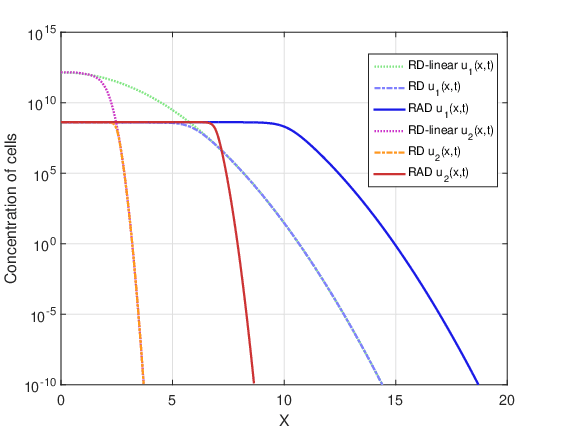
Influence of the nonlinear term on cell proliferation
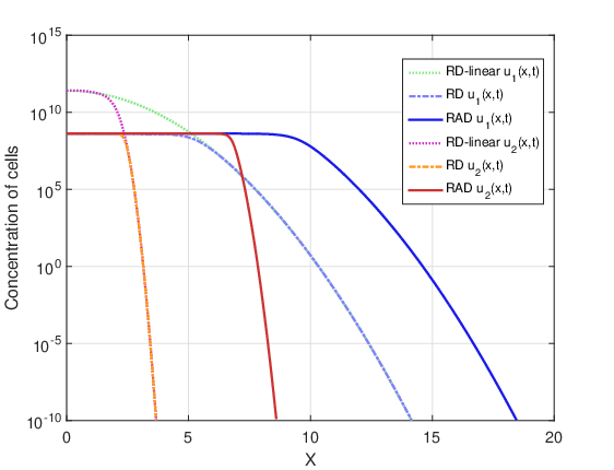
The previously presented results simulate the evolution of the glioma up to 80 days. However, this time is insufficient for the influence of the nonlinear term on the logistic proliferation to be noticed, since \(u(x,t) << u_{max}\) \(\forall t \l90\). Now, results of glioma evolution up to 720 days are presented for cases DOT \(=0\) day (without therapy) and DOT \(=5\) days (best therapy).
In this simulation, the RAD and RD models, equation (11) and (13), and the linear version of the RD model (called RD-linear) with \(u_{max} \to \infty\) were used. That is, in the RD-linear model there is no saturation limit for tumor cells. Thus, the RD model, equation (13) reduces to the RD-linear model defined by the equation (26)
(26)
\[ \dfrac{\partial \bar{u}}{\partial t} = D^{*} \dfrac{\partial^2 \bar{u}}{\partial x^2} + \bar{u}A^{*}.\]
Figures 12 and 13 show tumor cell concentration as a function of \(x\) predicted by RAD, RD and RD-linear models for \(t_f=720\) days and the two initial conditions \(u_1(x,0)\) and \(u_2(x,0)\). It is remarkable that, for both initial conditions, without the restrictive term \(u_{max}\) the cell concentration for the RD-linear model grows much more than for the RAD and RD models. For this reason, it was necessary to use the logarithmic scale to better visualize the results. The curves of the RAD and RD models do not grow beyond the saturation limit \(u_{max}\).
Figures 14 and 15 show the evolution of the maximum cell concentration over the days for the RAD, RD and RD-linear models with the two initial conditions. It can be observed that from day 600 onwards, the curves of the RD and RAD models present the constant value \(u_{max}\). However, the curve of the RD-linear model continues to grow almost exponentially for the two initial conditions. Also, it is observed that, approximately from day 340 for the case DOT \(=\) 0 day and from day 390 for the case DOT \(=\) 5 days, the growth of the RAD and RD models with the term nonlinear differs significantly from the RD-linear model.
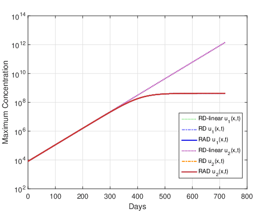
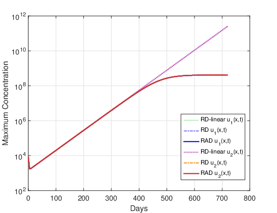
Clinically, it is common to use tumor “size” as a surrogate marker for overall survival (Dempsey et al., 2005). The exponential proliferation of glioma cells should not spontaneously cease until the tumor reaches its lethal size. It is well known that in this growth process there is competition between cells, such as competition for nutrients. Assuming that the final stage of this competition between malignant cells could be related to exponential growth saturation, it is reasonable to think that growth saturation has some relationship with the patient’s survival time. On the other hand, statistical data in the literature show that the average survival time for patients with glioma high-grade untreated tumor ranges from 6 months to 1 year. Whereas our simulations including the non-linear term estimate that the beginning of the glioma growth saturation process was approximately 1 year, it can be conjectured that the inclusion of this term in the model is fundamental to adequately estimate the patient’s survival time. It should be clear that this is just a conjecture, as glioma growth is a very complex biological phenomenon and is still not well understood. In other words, it is observed that for the input data considered in these simulations, the saturation process in glioma growth starts approximately after 1 year, and this non-linear term can be crucial to adequately estimate the patient’s survival time. Although this term was known to us, it had not been considered in our previous studies, since it was not included in the analyzes carried out by Barbosa et al., 2019, Jesus et al., 2014, Silva et al., 2016 and Souza et al., 2015.
Conclusions
This work analyzes the influence of the terms of a reactive-advective-diffusive PDE used to model the evolution of gliomas. A combined RAD model is constructed and compared with the RD and RD-linear models. In this way, comparing the solutions of all models, it is possible to estimate the influence of each term.
These three continuous models were discretized using the finite difference method. All spatial derivatives at interior points of the domain were discretized with centered second-order differences. For the boundary points forward and backward second-order differences were used. A first-order direct difference was used for the non-linear term in cell proliferation. After linearizing the PDE, the Crank-Nicolson method was applied considering only the reactive-diffusive terms, while the advective term was approximated using the upwind method.
Simulation results are shown for four scenarios: no radiotherapy, application of a single dose, and two dose fractionation schemes. By simple comparison, it is possible to verify that the fractionation of the dose presents therapeutic advantages, as is already widely recognized in the literature. Also, it was found that the RAD model is more dispersive than the RD model, since in addition to the diffusive term the advective term contributes to cell mobility. This means that the tumor radius for the RAD model is always larger than for the RD model.
It was found that, generally, the evolution of the tumor radius has three stages: first an oscillatory decrease caused by treatment with fractioned doses, second a period of recession where the tumor radius is below the detection threshold, and third, the resumption of tumor growth after the end of the effects of the treatment. In case of non-use of radiotherapy the tumor radius hardly grows. In the case of very small dose fractions like DOT \(=\) 35 days the recession period does not occur.
When comparing the results of the RAD and RD models for maximum concentration of tumor cells, it is verified that they are both equal. The reason for this is that the advective term in the RAD model neither creates nor destroys tumor cells. It is also concluded that the maximum concentration of tumor cells always decreases during the application of the treatment and increases again at the end of the treatment. The decreasing region in the maximum cell concentration plot has a “sawtooth” shape that depends on the fractioned dose value. The DOT \(=\) 35 days treatment showed a smaller reduction in tumor radius without recession period. The DOT \(=\) 5 days treatment showed the greatest reduction in tumor radius and the longest period of recession, offering a longer window of time for the medical team to apply another type of therapy, such as surgical resection or chemotherapy.
Comparing the predictions of the RAD and RD models for the two analyzed initial conditions, it is possible to observe that for some cases of fractionation there are significant differences. For the initial condition \(u_1(x,0)\) the growth in the RAD and RD models is always almost exponential after the end of the treatment effects. However, for the initial condition \(u_2(x,0)\) both models show two significant changes in the growth rate of the tumor radius after the end of the treatment effects. Everything indicates that these changes are related to the initial radius of the tumor \(R_0\) and the different parts of the initial condition \(u_2(x,0)\). In the RAD model, these two changes in growth rate occur at earlier time points than in the RD model, and this can be explained by the fact that the RAD model has a greater dispersion of cells than the RD model. Only in the cases DOT \(=\) 0 day and DOT \(=\) 35 days it was not possible to observe these two changes in the growth rate for the initial condition \(u_2(x,0)\). Furthermore, for all fractionation schemes in the two models, it is verified that, after the end of the treatment effects, the tumor radius predicted by the initial condition \(u_2(x,0)\) is always smaller than that predicted by \(u_1( x,0)\). Considering that the shape of the two initial conditions is very similar, and that the main difference between these two initial conditions lies in the continuity of the first derivative, we can conclude that the analyzed models are sensitive to the mathematical properties of the initial condition. This justifies the need for further studies on which initial condition should be used so that the mathematical model is as close as possible to reality.
Finally, it was found that without the non-linear term of cell proliferation, glioma growth is unlimited, which does not occur in practice. Whereas statistical data in the literature show that the average survival time for patients with glioma high-grade untreated tumor ranges from 6 months to 1 year, and that our simulations including the non-linear term estimate that the beginning of the glioma growth saturation process was approximately 1 year, it can be concluded that the inclusion of this term in the model may be fundamental to properly estimate the patient’s survival time. Our arguments for this conjecture were presented at the end of the previous section.
Author Contributions
B.S. Alvarez and G.B. Lobão, D.C. participated in the: Conceptualization, Data Curation, Formal Analysis, Methodology, Project Management, Resources, Programs: Machado. Alvarez, G.B. and Lobão, D.C. participated in the: Supervision. Machado, B.S. and Alvarez, G.B. participated in the: Research, Validation, Visualization, Writing - preparation of the original draft, Writing – revision and editing.
Conflicts of interest
Not applicable.
Acknowledgments
This work was supported by the Universidade Federal Fluminense. The authors are grateful for the constructive comments made by the reviewers.
References
S. K. Aggarwal (1985). Some numerical experiments on fisher equation. 12(4), 417-430. https://doi.org/10.1016/0735-1933(85)90036-3
Barbosa, O. X., Assis, W. L. S., Garcia, V. S. & Alvarez, G. B. (2019). Computational simulation of gliomas using stochastic methods. Cajazeiras. 199-215. https://doi.org/10.29215/pecen.v3i2.1285
Dempsey, Mary F., Condon, Barrie R. & Hadley, Donald M. (2005). Measurement of Tumor “Size” in Recurrent Malignant Glioma: 1D, 2D, or 3D?. 26(4), 770--776.
Eric J. Hall (2000). Radiobiology for the Radiologist. Lippincott Williams & Wilkins.
Michael C. Joiner & Albert J. van der Kogel (2009). Basic Clinical Radiobiology. Taylor & Francis Group.
Jesus, J. C., Christo, E. S., Garcia, V. S. & Alvarez, G. B. (2014). Time Series Analysis For Modeling Of Glioma Growth In Response To Radiotherapy. Canadá. 14(3), 1532-1537. https://doi.org/10.1109/TLA.2016.7459646
Leder, K., Pitter, K., Laplant, Q., Hambardzumyan, Dolores, Ross, Brian D., Chan, Timothy A., Holland, Eric C. & Michor, Franziska (2014). Mathematical modeling of PDGF-driven glioblastoma reveals optimized radiation dosing schedules. Cambridge. 156(3), 603--616. https://doi.org/10.1016/j.cell.2013.12.029
Machado, Bruno Silva (2023). Estudo e Análise Numérica de Modelos Reativo-Advectivo-Difusivo para o Crescimento de Gliomas Tratados com Radioterapia.
Rockne, R., Alvord, E. C., Rockhill, J. K. & Swanson, K. R. (2009). A mathematical model for brain tumor response to radiation therapy. New York. 58(4-5), 561-578. https://doi.org/10.1007/s00285-008-0219-6
Shuman, R. M.,, Alvord, E. C., & Leech, R. W. (1975). The biology of childhood ependymomas. American Medical Association. 32(11), 731-739. https://doi.org/10.1001/archneur.1975.00490530053004
Junior Jose Silva (2014). Modelagem Computacional Aplicada ao Tratamento de Câncer Via Medicina Nuclear.
Silva, Júnior José, Alvarez, G. B., Garcia, V. S. & Lobão, D. C. (2016). Modelagem Computacional do Crescimento de Glioma via Diferenças Finitas em Resposta à Radioterapia. 36 Congresso Nacional de Matemática Aplicada e Computacional, Gramado. https://doi.org/10.5540/03.2017.005.01.0327
Silva, Larissa Miguez, Alvarez, Gustavo Benitez, Christo, Eliane Silva,, Pelén Sierra, Gerardo Amado & Garcia, Vanessa Silva (2021). Time series forecasting using ARIMA for modeling of glioma growth in response to radiotherapy. 42(1), 3–12. https://doi.org/10.5433/1679-0375.2021v42n1p3
Souza, E. B., Alvarez, G. B., & Neves, T. A. (2015). Estudo sobre otimizaçao da radioterapia em pacientes com gliomas. In: SIMPOSIO BRASILEIRO DE PESQUISA OPERACIONAL, 47., 2015, Porto de Galinhas. Proccedings of SBPO. Porto de Galinhas: SBPO Publishing .
Souza, E. B., Alvarez, G. B., & Neves, T. A. (2015). Estudo sobre otimizaç\~ao da radioterapia em pacientes com gliomas.. 47 Simpósio Brasileiro de Pesquisa Operacional, Porto de Galinhas..
Stein, Andrew, Demuth, Tim, Mobley, David, Berens, Michael & Sander, Leonard (2007). A Mathematical Model of Glioblastoma Tumor Spheroid Invasion in a Three-Dimensional In Vitro Experiment. Elsevier. 356-65. https://doi.org/10.1529/biophysj.106.093468
Kristin R. Swanson, Carly Bridge, J. D. Murray & Ellsworth C. Alvord (2003). Virtual and real brain tumors: using mathematical modeling to quantify glioma growth and invasion. Elsevier. 216(1), 1-10. https://doi.org/10.1016/j.jns.2003.06.001