
Numerical Simulation of the Production of Core-Shell Microparticles
Fernandes, C.; Ferrás, L. L.; Afonso, A. M.
DOI 10.5433/1679-0375.2023.v44.47206
Citation Semin., Ciênc. Exatas Tecnol. 2023, v. 44: e47206
Abstract:
Conventional methods that are commonly used for the preparation of microbubble delivery systems include sonication, high–shear emulsification, and membrane emulsification. However, these methods present significant disadvantages, namely, poor control over the particle size and distribution. To date, engineering core–shell microparticles remains a challenging task. Thus, there is a demand for new techniques that can enable control over the size, composition, stability, and uniformity of microparticles. Microfluidic techniques offer great advantages in the fabrication of microparticles over the conventional processes because they require mild and inert processing conditions. In this work, we present a numerical study based on the finite volume method, for the development of capsules by considering the rheological properties of three phases, air, a perfluorohexane (\(C_{6}~F_{14}\)) and a polymeric solution constituted of a solution of 0.25% w/v alginate. This methodology allows studying the stability and behavior of microparticles under different processing conditions.
Keywords: numerical methods, numerical simulation, finite volume method, free-surface, core-shell particles
Introduction
Core-shell particles are particles having a core of one material and a shell of a different material, see Figure 1.

As a result of their potential for drug delivery, biomedical imaging, tumour therapy, and microfluidic devices, core–shell particles have become increasingly important in the past decade (Galogahi et al., 2020; Jenjob et al., 2020; Mahdavi et al., 2020). A combination of these two materials at nano and micro-scales has also facilitated the development of innovative technologies in many areas of science, resulting in a new field of micro-strategies for the development and design of biological devices and systems (Mahdavi et al., 2020).
Sonication, high shear emulsification, and membrane emulsification are all typical ways for producing microbubbles (Chen et al., 2014; Stride & Edirisinghe, 2008). These approaches, however, have substantial limitations, including limited control over particle size and dispersion. As a result, new strategies for controlling the size, composition, stability, and homogeneity of microparticles are required.
Because they need mild and inert processing conditions, microfluidic procedures offer substantial advantages over conventional methods for manufacturing microparticles. Furthermore, the size dispersion of particles produced by microfluidic devices is constrained. Despite the fact that multiple research groups have recorded the production of alginate particles using various microfluidic devices (Zhang et al., 2021), few have reported the production of capsules or core-shell particles, particularly employing a microfluidic glass capillary device (Hayes et al., 2014).
Therefore, in this work, we numerically study the process of formation of core-shell particles. This way we can easily change the characteristics of the process, and infer the stable conditions for the production of different microparticles. Based on the experimental work of Duarte et al., 2014, we focus on the application of alginate (a biopolymer derived from sea algae, that has been described for a large number of pharmaceutical and biomedical applications because of its biocompatibility and ease of gelation) as a shell, and a core made of a perfluorocarbon (PFC), namely a perfluorohexane (\(C_{6}~F_{14}\)). The other medium is air.
A schematic of the experimental apparatus is shown in Figure 2.

The PFC is injected through a narrow microchannel (cappilary 1) that is inside another microchannel (cappilary 2) filled with the polymer solution (alginate). The narrow microchannel injects PFC to the polymer solution medium. When cappilary 2 ends, the micro-particles become in contact with air, and a core-shell microparticle is formed.
The sections in this paper are as follows. In section Governing equations we introduce the basic equations governing the flow of a multiphase fluid, while in section Numerical method the numerical methodology used to discretize the governing equations is explained. In section Geometry, mesh and fluids properties the geometry and meshes used in the simulations are presented and the fluids properties are defined. Subsequently, in section Results and discussion we present the numerical results obtained for different flow conditions. Finally, section Conclusions presents the contributions of the paper.
Governing equations
Numerical simulations of the microbubble delivery system phenomena are performed using an advanced free-surface capturing model based on a two-fluid formulation of the classical volume-of-fluid (VOF) model (Rusche, 2002) in the framework of the finite volume method (FVM) (OpenCFD, 2007). In this model an additional convective term is introduced into the transport equation for phase fraction, contributing decisively to a sharper interface resolution.
In the conventional VOF method (Hirt & Nichols, 1981) the transport equation for an indicator function, representing the volume fraction of one phase, equation (1), is solved simultaneously with the continuity and momentum equations, equations (2) and (3),
(1)
\[ \frac{\partial\gamma}{\partial t}+\nabla\cdot(\textbf{U}\gamma) = 0,\]
(2)
\[ \nabla \cdot \textbf{U} = 0,\]
(3)
\[ \frac{\partial(\rho\textbf{U})}{\partial t}+\nabla\cdot(\rho\textbf{UU}) = -\nabla p + \nabla \cdot \textbf{T} + \rho\textbf{f}_b,\]
where \(\textbf{U}\) represents the velocity field shared by the fluids (equal or greater than two) throughout the flow domain, \(\gamma\) is the phase fraction, \(\textbf{T}\) is the deviatoric viscous stress tensor (\(\textbf{T}=2\mu \textbf{S}-2\mu (\nabla\cdot\textbf{U})\textbf{I}/3\), with \(\mu\) being the fluid dynamic viscosity, \(\textbf{S}=0.5[\nabla\textbf{U}+(\nabla\textbf{U})^T]\) being the mean rate of the strain tensor and \(\textbf{I}=\delta_{ij}\) is the identity tensor defined using the Kronecker delta), \(\rho\) is density, \(t\) is time, \(p\) is pressure, and \(\textbf{f}_b\) are body forces per unit mass. Usually, in VOF simulations the body forces considered are gravity and surface tension effects at the interface. The phase fraction \(\gamma\) can take values within the range \(0\leq \gamma \leq 1\), with the values of zero and one corresponding to regions accommodating only one phase. As a consequence, gradients of the phase fraction are found only in the interface region.
The methodology presented hereafter considered only two fluids but can be extended to a finite number of fluids (Faghri & Zhang, 2006). Thus, we consider two immiscible fluids as one effective fluid throughout the domain. For the effective fluid the physical properties are calculated as weighted averages based on the distribution of the liquid volume fraction,
(4)
\[ \rho=\rho_1 \gamma+\rho_2(1-\gamma),\]
(5)
\[ \mu=\mu_1 \gamma+\mu_2(1-\gamma),\]
where \(\rho_1\) and \(\rho_2\) are densities of fluid one and fluid two, respectively, and \(\mu_1\) and \(\mu_2\) are dynamic viscosity’s of fluid one and fluid two, respectively. When simulating free surface flows using the VOF model, the conservation of the phase fraction is of major importance, namely for a proper evaluation of surface curvature, which is required for the determination of surface tension force and the corresponding pressure gradient across the free surface.
In the present study a modified approach similar to the one proposed in (Rusche, 2002) is used, with an advanced model formulated by OpenCFD, 2007 Ltd., relying on a two-fluid formulation of the conventional VOF model in the framework of the FVM. First, phase fraction equations are solved separately for each individual phase as in the two-fluid Eulerian model (Cerne et al., 2001). Equations for each of the phase fractions can be expressed as,
(6)
\[ \frac{\partial\gamma}{\partial t}+\nabla\cdot(\textbf{U}_{1} \gamma) = 0,\]
(7)
\[ \frac{\partial(1-\gamma)}{\partial t}+\nabla\cdot(\textbf{U}_{2} (1-\gamma)) = 0.\]
Defining the velocity of the effective fluid in a VOF model as a weighted average,
(8)
\[\begin{aligned} \textbf{U} & = & \gamma \textbf{U}_{1}+(1-\gamma)\textbf{U}_{2}, \end{aligned}\] and assuming that the contributions of both fluids velocities to the evolution of the free surface are proportional to the corresponding phase fraction, equation (6) can be rearranged to obtain the evolution equation for the phase fraction \(\gamma\),
(9)
\[\begin{aligned} \frac{\partial\gamma}{\partial t}+\nabla\cdot(\textbf{U}\gamma)+\nabla\cdot[\textbf{U}_{r} \gamma(1-\gamma)] & = & 0, \end{aligned}\]
where \(\textbf{U}_{r}=\textbf{U}_{1}-\textbf{U}_{2}\) is the vector of relative velocity, called as the “compression velocity". The additional convective term contributes significantly to a higher interface resolution, thus avoiding the need to devise a special scheme for convection, such as the CICSAM (Ubbink & Issa, 1999). Details of “compression velocity" numerical treatment are given in section Numerical method.
The effects of surface tension should be introduced in the momentum equation, equation (3). The surface tension at the interface generates an additional pressure gradient resulting in a force, which is evaluated per unit volume using the continuum surface force (CSF) model (Brackbill et al., 1992),
(10)
\[\begin{aligned} \textbf{f}_{\sigma} & = & \sigma\kappa\nabla\gamma, \end{aligned}\]
where \(\sigma\) is the interfacial surface tension and \(\kappa\) is the mean curvature of the free surface, determined from the expression,
(11)
\[\begin{aligned} \kappa & = & -\nabla \cdot \left(\frac{\nabla\gamma}{|\nabla\gamma |}\right). \end{aligned}\]
All the fluids considered in this work are Newtonian and incompressible. Thus, the rate of strain tensor is linearly related to the stress tensor, which is written into a more convenient form for discretization,
(12)
\[\begin{aligned} \nabla\cdot\textbf{T} &= \nabla\cdot\left[\mu(\nabla \textbf{U} + (\nabla\textbf{U})^T)\right] \nonumber \\ &= \nabla\cdot(\mu\nabla\textbf{U})+ (\nabla\textbf{U})\cdot\nabla\mu. \end{aligned}\]
As the VOF method presented here is formed by a single pressure system, the normal component of the pressure gradient at a stationary non-vertical solid wall, with no-slip condition on velocity, must be different for each phase due to the hydrostatic component \(\rho g\) when the phases are separated at the wall, i.e., if a contact line exists. In order to simplify the definition of boundary conditions, it is common to define a modified pressure as,
(13)
\[\begin{aligned} p_{d} & = & p-\rho\textbf{g}\cdot \textbf{x}, \end{aligned}\] where \(\textbf{g}\) is the gravitational acceleration vector and \(\textbf{x}\) is the position vector. In order to satisfy the momentum equation, equation (3), the pressure gradient is expressed using equation (13). Therefore, momentum equation is rearranged to give (Rusche, 2002)
(14)
\[\begin{aligned} & \frac{\partial(\rho\textbf{U})}{\partial t}+\nabla\cdot(\rho\textbf{UU})- \nabla\cdot(\mu\nabla\textbf{U})-(\nabla\textbf{U})\cdot \nabla\mu \nonumber \\ &= -\nabla p_{d} - \textbf{g}\cdot\textbf{x} \nabla \rho + \sigma\kappa\nabla\gamma. \end{aligned}\]
The global mathematical model is given by the continuity equation, equation (2), phase fraction equation equation (9), and momentum equation equation (14). These equations allow to compute the dynamic pressure (\(p_d\)), velocity components (\(\textbf{U}\)) and distribution of the liquids (\(\gamma\)) inside the two-phase flow. The non-linearities present in these equations, coming from the advective terms, are first linearized using an explicit construction of the flux (Jasak, 1996).
Numerical method
An open source computational fluid dynamics (CFD) framework code, \(OpenFOAM^®\) (Weller et al., 1998), was used in this study. The code is based in a cell-center finite volume method on a fixed unstructured numerical grid. The coupling between pressure and velocity fields in transient flows is done by employing the pressure implicit with splitting of operators (PISO) algorithm (Issa, 1986).
The finite volume technique is used for discretization of the governing equations presented in section Governing equations. The source terms are discretized using the midpoint rule and integrated over cell volumes. The implicit Euler scheme is used for the discretization of the time derivative terms. The spacial derivatives terms (diffusion and convective terms) are converted into surface integrals bounding each cell making use of Gauss theorem. The cell faces values are obtained by interpolation and then summed up to obtain the surface integral. For the evaluation of gradients a linear face interpolation is used.
The compression term in equation (9) is discretized using the relative velocity at cell faces, which are based on the maximum velocity magnitude at the interface region and its direction. Hence, the gradient of phase fraction is used to compute the relative velocity at cell faces as,
(15)
\[\begin{aligned} U_{r,f}&=&n_{f} \texttt{min} \left[C_{\gamma}\frac{|\phi|}{|\textbf{S}_{f}|}, \texttt{max}\left(\frac{|\phi|}{|\textbf{S}_{f}|}\right)\right], \end{aligned}\]
where \(\phi\) is face volume flux, \(C_{\gamma}\) is the intensity of the free surface compression, \(\textbf{S}_{f}\) is the surface area vector, and \(n_{f}\) is the face unit normal flux, calculated at cell faces in the interface region using the phase fraction gradient at cell faces,
(16)
\[\begin{aligned} n_{f}&=&\frac{(\nabla\gamma)_{f}}{|(\nabla\gamma)_{f}+\delta_{n}|}\cdot \textbf{S}_{f}. \end{aligned}\]
In order to account for non-uniformity of the grid, a stabilization factor \(\delta_{n}\) is used in the normalization of the phase fraction gradient in equation (16),
(17)
\[\begin{aligned} \delta_{n}&=&\frac{\epsilon}{\left(\dfrac{{\sum\limits_{N}} V_i} {N}\right)^{1/3}}, \displaystyle\frac{\epsilon}{\left(\displaystyle\frac{\displaystyle\sum_{N}V_{i}}{N}\right)^{1/3}}, \end{aligned}\]
where \(N\) is the number of computational cells, each one with own volume \(V_i\), and \(\epsilon\) is a small parameter (defined as \(10^{-8}\)).
The OpenFOAM framework is capable of doing adaptive time step control in order to ensure stability of the solution procedure. The time step is adjusted at the beginning of the time iteration loop based on the Courant number defined as,
(18)
\[\begin{aligned} Co&=&\frac{|\textbf{U}_{f}\cdot \textbf{S}_{f}|}{\textbf{d}\cdot \textbf{S}_{f}}\Delta t, \end{aligned}\]
where \(\textbf{d}\) is a vector joining the control volumes centroids sharing the same face and \(\Delta t\) is time step. Using values for \(\textbf{U}_{f}\) and \(\Delta t\) from previous time step, a maximum local Courant number \(Co^{0}\) is calculated and the new time step is given by
(19)
\[\begin{aligned} \Delta t^{n}&=&\texttt{min}\left\lbrace A,B,\lambda_{2}\Delta t^{0},\Delta t_{max}\right\rbrace, \end{aligned}\]
where \(A=\dfrac{Co_{max}}{Co^{0}}\Delta t^{0}\) and \(B=\left(1+\lambda_{1}\dfrac{Co_{max}}{Co^{0}}\right)\Delta t^{0}\). \(\Delta t_{max}\) and \(Co_{max}\) are user-defined limit values for the time step and Courant number, respectively. The increase of the time step is damped using factors \(\lambda_{1}\) and \(\lambda_{2}\).
During the first runs it was found that the limit value for the Courant number should not exceed \(Co_{max}=1.0\), which is the value also used in this study. The size of the time steps was varying during calculations between values on the order of \(10^{-9}\) s to \(10^{-7}\) s.
In addition, the OpenFOAM framework solves the phase fraction equation in several subcycles, \(n_{sc}\), within a single time step, \(\Delta t\). Thus, the time step to be used in a single time subcycle is computed as,
(20)
\[\begin{aligned} \Delta t_{sc}&=&\frac{\Delta t}{n_{sc}}. \end{aligned}\]
In each subcycle the phase fraction \(\gamma\) is computed and the corresponding mass flux \(F_{sc,i}\) through cell faces is obtained. Afterwards, the total mass flux \(F\) of the global time step, which is needed in the momentum equation, is computed with the following equation,
(21)
\[\begin{aligned} F&=&\rho \textbf{U}_{f}\cdot \textbf{S}_{f}=\displaystyle\sum_{i=1}^{n_{sc}}\frac{\Delta t_{sc}}{\Delta t}F_{sc,i}. \end{aligned}\]
With this algorithm a more accurate solution of the phase fraction equation is obtained and, also, it enables the use of a greater global time step size for the solution of other transport equations, which can speed up the solution procedure.
For a detailed analysis of the discretized governing equations modelling two-phase incompressible flows in the OpenFOAM framework the reader should refer to (Deshpande et al., 2012).
Geometry, mesh and fluids properties
Figure 3 shows a schematic diagram of the three-phase glass capillary model used in this study. The computational domain was simplified taking into account that the model is axisymmetric. The geometry consisted of four concentric glass capillaries. The first capillary (capillary 1) has an inner diameter (ID) of 50 \(\mu m\), the second capillary (capillary 2) has an ID of 150 \(\mu m\), the third glass capillary (capillary 3) has an ID of 800 \(\mu m\), and the outer glass capillary (capillary 4) has an ID of 1450 \(\mu m\). The geometry has been designed to allow the coaxial flow of three different solutions in each capillary more one capillary mimicking the atmosphere (see also Figure 2.

The inner fluid was a perfluorocarbon (PFC), namely, perfluorohexane (\(C_{6}~F_{14}\)). Perfluorohexane has a boiling point above room temperature, 57 \(^{\circ}\)C, and a vapor pressure of 27 kPa. This volatile liquid PFC was selected in order to enhance particle stability and prevent the coalescence of the particles. The middle aqueous phase was the polymeric solution (PS), constituted of a solution of 0.25% w/v alginate. Table 1 lists the density and viscosity of all phases. The interfacial surface tension used for all three interactions (air-PS, air-PFC and PS-PFC) was defined as \(0.07~N/m\).
| Phase | Density (\(kg/m^3\)) | Viscosity (\(mPa s\)) |
|---|---|---|
| Inner phase (PFC) | 1669 | 0.67 |
| Middle phase (PS) | 1002.5 | 5.31 |
| Outer phase (AIR) | 1 | 0.0148 |
The boundary conditions are summarized as follows. In the inlets of the first and second fluid the mass flow rate was imposed, in the third inlet the air flow was generated by a prescribed pressure and in the fourth inlet no air flow was generated. At the outlet a pressure outlet was imposed. At the symmetry axis a wedge type boundary condition was specified and in the walls a no-slip boundary condition was chosen.
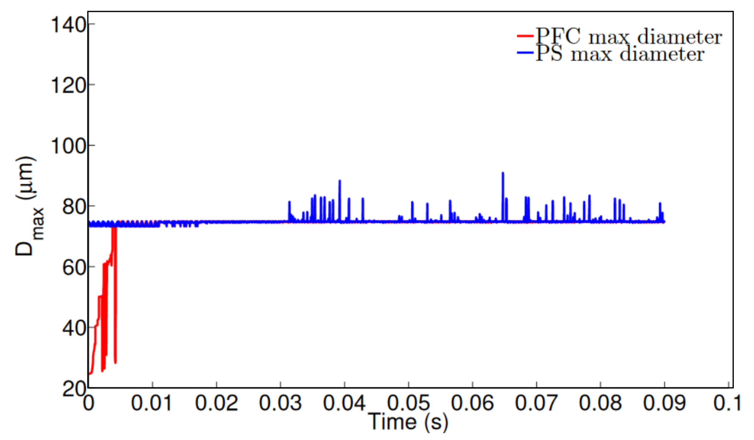
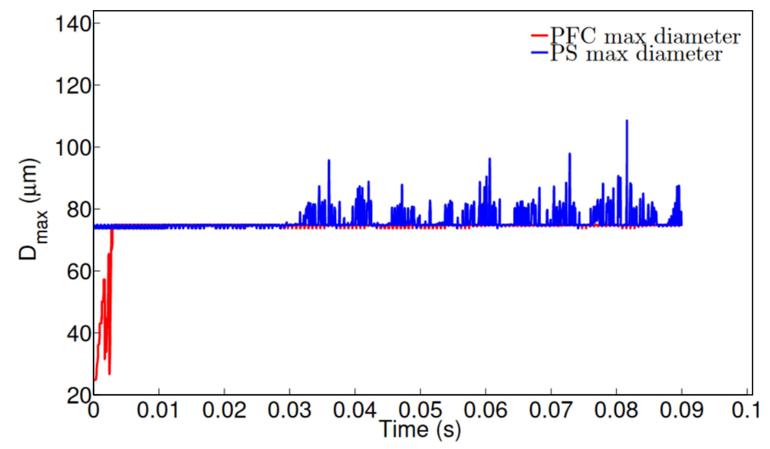
A grid dependency study was performed by considering four meshes with a resolution of \(10, 7.5, 5\) and \(2.5~\mu m\) in the \(x\) direction and \(40, 30, 20\) and \(10~\mu m\) in the \(z\) direction.
(a)
(b)
(a)
(b)
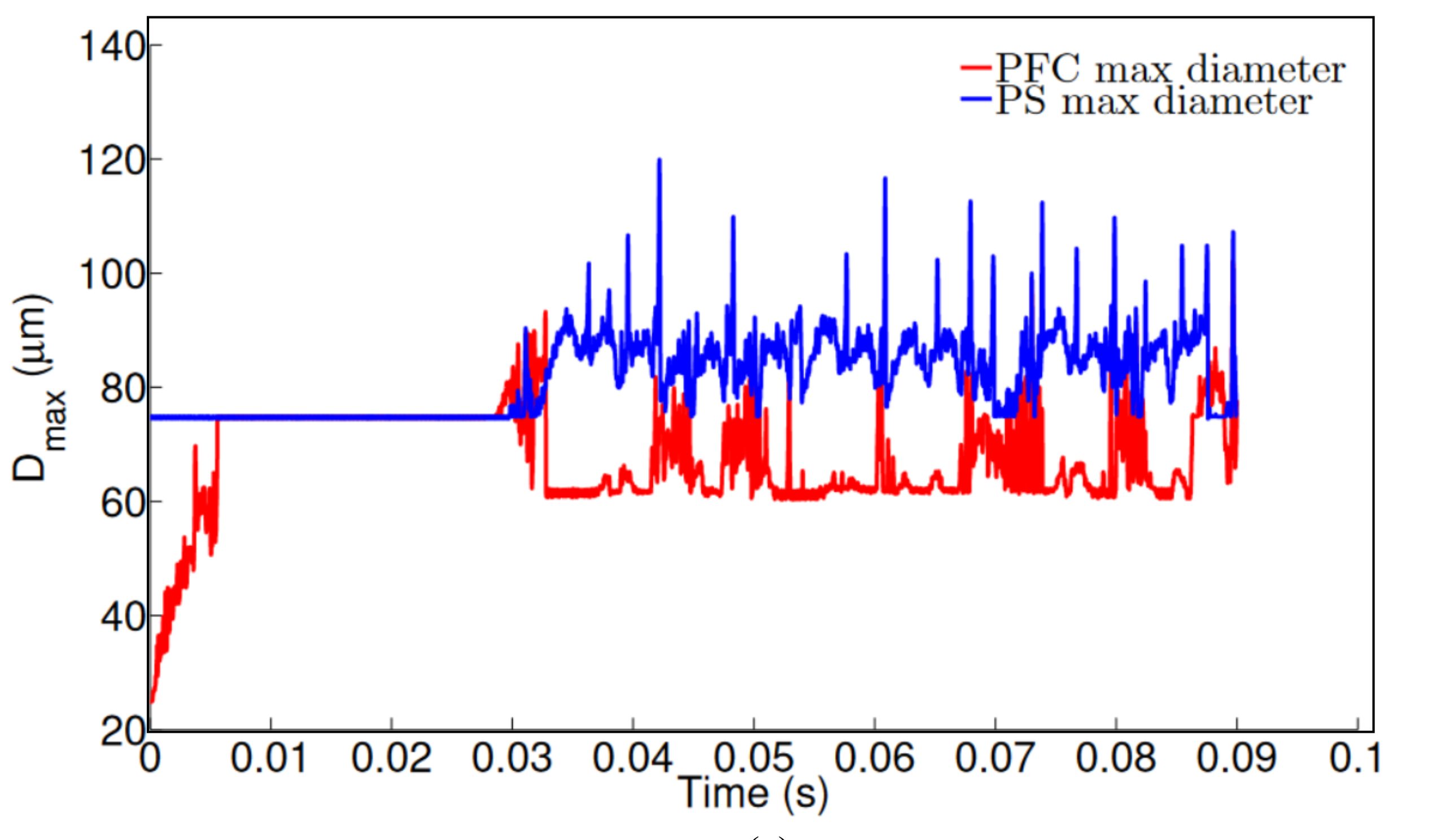
Figure 4 shows the results for both inner and middle phases maximum droplet diameter, considering the two less refined meshes (Mesh 1 and Mesh 2). The conditions imposed on the simulation were flow rates of 10 and 50 \(\mu L/min\) for PFC and PS, respectively, and pressure air flow of 200 \(Pa\). It is seen that this mesh resolution is not sufficiently accurate to predict both core and shell diameters. There are changes in the order of \(50\mu m\), when going from Mesh 1 to Mesh 2.
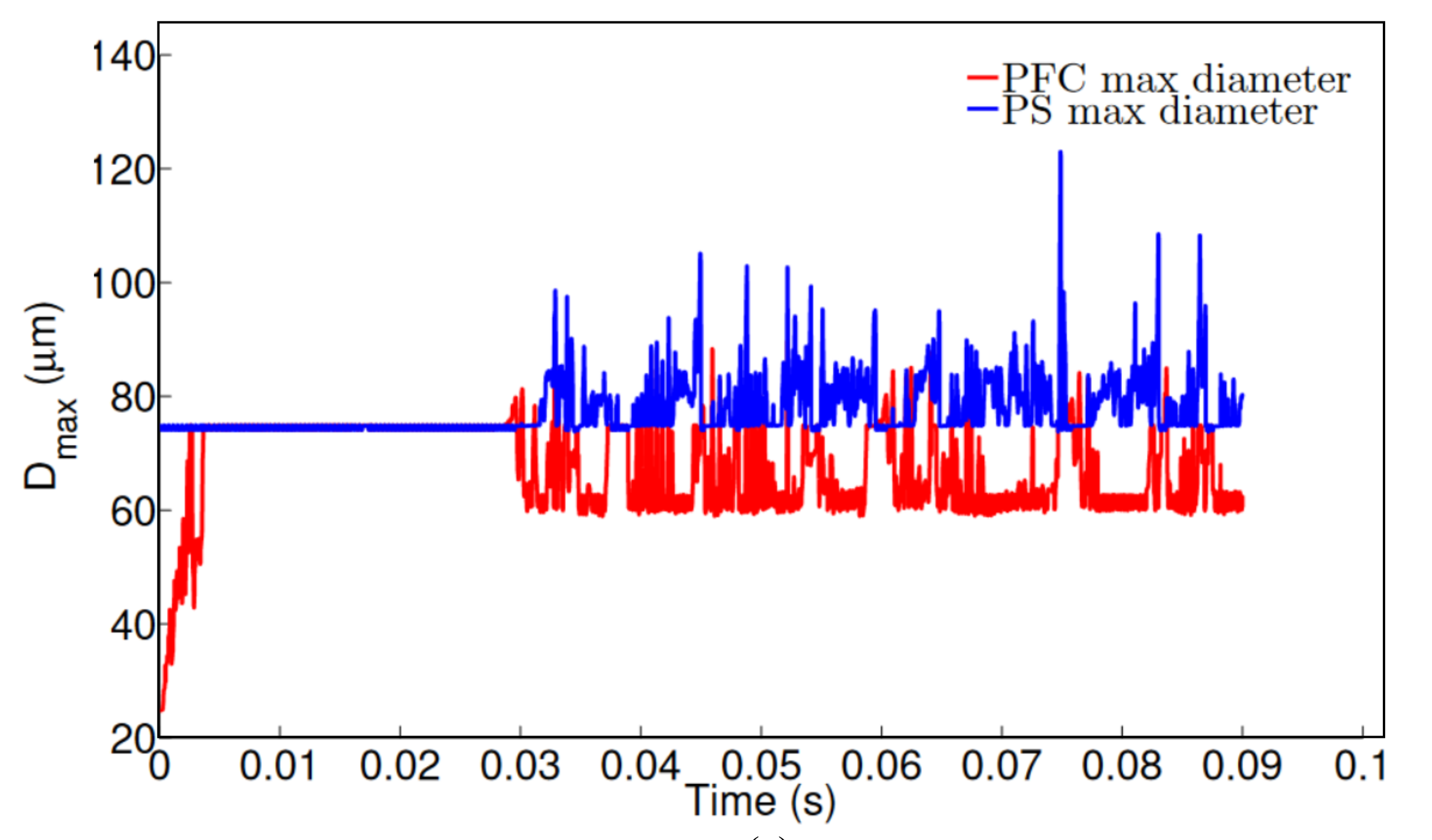
The results obtained for Mesh 3 and Mesh 4 are shown in Figure 5. We now see a small difference in behavior between the results obtained with Mesh 3 and Mesh 4. The ranges of PFC and PS maximum diameter’s are very similar. Hence, Mesh 3 is selected to be used on the subsequent studies due to less computational efforts comparing with Mesh 4.
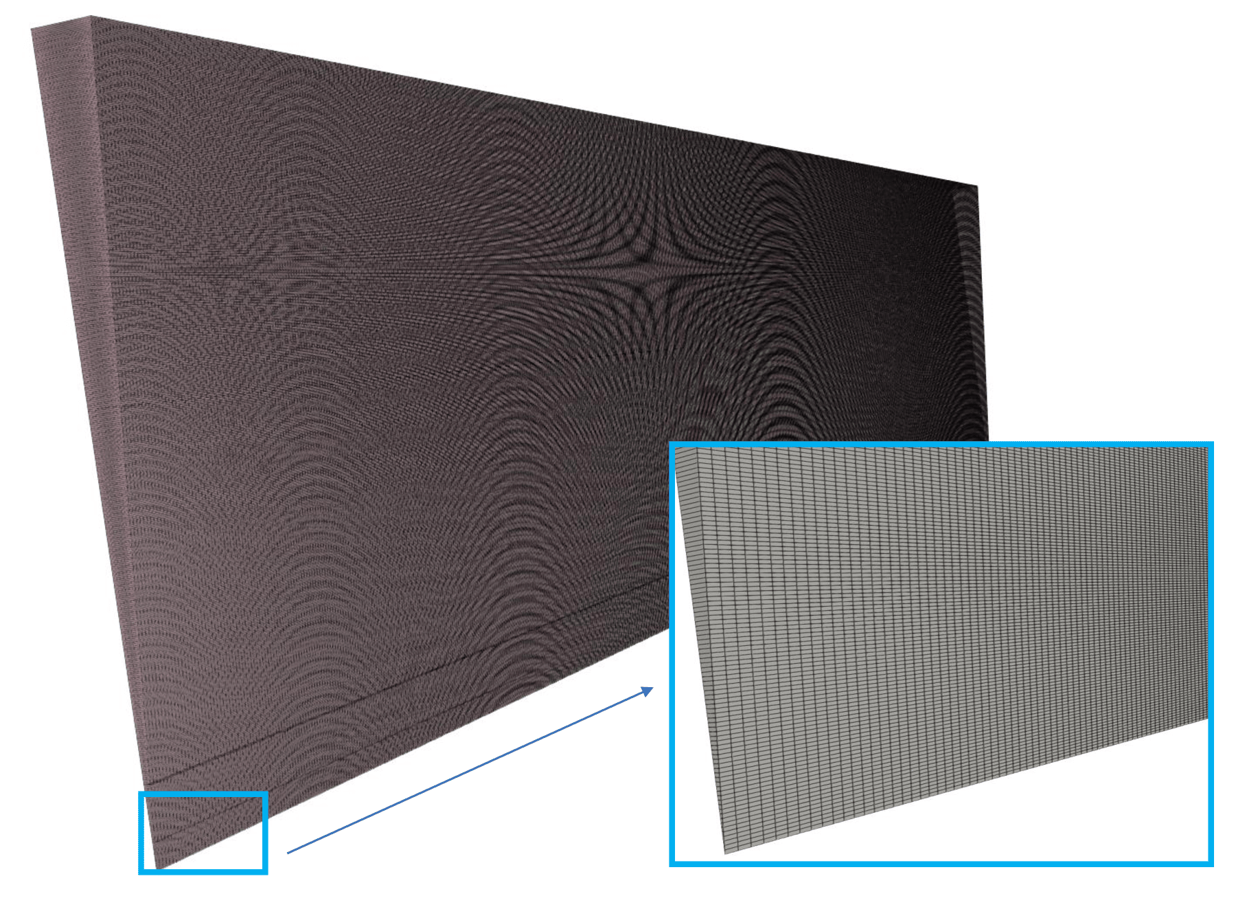
Figure 6 shows a zoomed view of Mesh 3, where we have 417600 cels (416880 hexahedra and 720 prisms-adjacent to the axis of symmetry).
Results and discussion
The numerical tests performed followed the experimental work of Duarte et al., 2014. It should be noted that experimentally the different capillaries have an inner and an outer diameter. The inner capillary has ID of \(50\mu m\) and an outer diameter (OD) of \(80\mu m\), the middle capillary has an ID of \(150\mu m\) and an OD of \(250\mu m\), and the outer glass capillary tube has an ID of \(800\mu m\). This results in a thickness of \(30\mu m\) for capillary 1 and \(100\mu m\) for capillary 2. In the simulations, we have only an inner diameter, and the thickness of the capillary is zero in all cases.
The experiment (Duarte et al., 2014) allows to control the pressure prevailing in the system and thus to compress the air. The flow rate of the injected air can also be adjusted. The authors concluded that increasing the pressure in the system (increasing the air inlet flow rate and keeping the amount of air leaving the system constant) leads to a decrease in particle size.
In our simulation, we can control the flow rate of the injected air (or impose a specific pressure at the inlet and outlet). Due to the difficulty in obtaining numerical convergence for highly pressurised systems, we will compare the results of our simulations with the experimental case of low pressure (5 PSI).
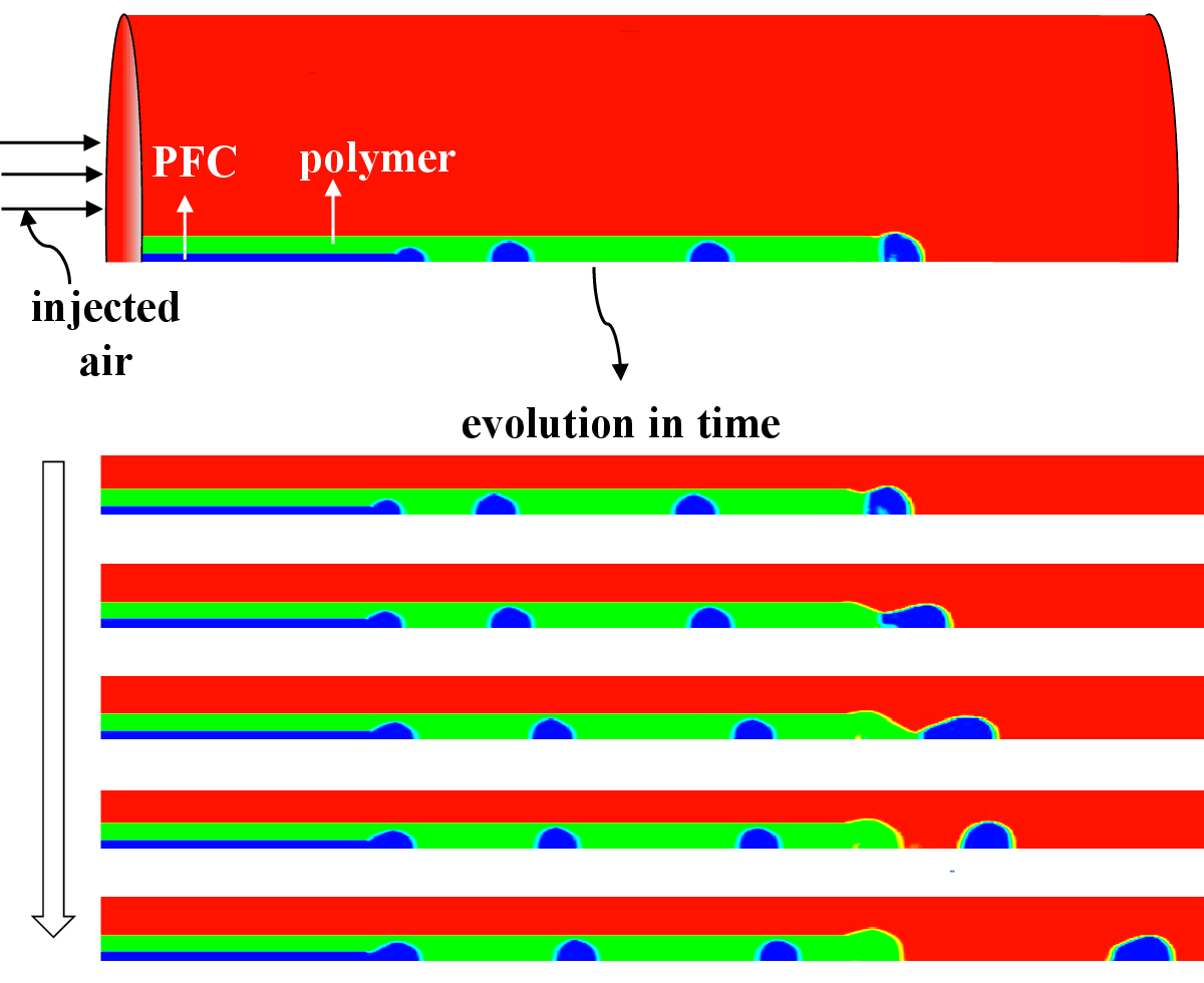
Case study:
Flow rates of 10 and 50 \(\mu L/min\) for PFC and PS, respectively, inlet imposed pressure (for air flow) of 200 \(Pa\) and outlet imposed pressure of 0 \(Pa\).
Note that the pressure imposed numerically results in a lower pressure than the internal pressure considered in the experimental system. Although, since the experimental pressure is low, we do not expect a big difference in the results.
The case study is illustrated in Figure 7. The upper part of the figure shows the complete geometry, the lower part shows a section of the region where the particles originate (the temporal evolution is shown). At these flow rates, there are three bubbles of PFC in capillary 2 (the capillary containing the polymer solution). As the particles approach the exit of capillary 2, the influence of the injected air is felt and the particles expand. Note that, as experimentally predicted, a core-shell of PFC (core) and the polymer solution (solution) is formed. This can be seen clearly in the last two time snaps.
A comparison between the experimental and numerical results is shown in Figure 8. In both the experimental and numerical results, we can easily distinguish the core and the shell. However, the results can only be compared qualitatively. The diameter of the particle in the numerical simulation is \(\approx 105 \mu m\), while in the experimental results it is \(\approx 124 \mu m\). These results may vary in both the experimental and numerical cases because the size of the core shell may change during the process. Numerically, we observed that the particle diameter is between 80 and 120 \(\mu m\), while experimentally it is between 110 and 130 \(\mu m\).

The experimental part of the figure was adapted from Duarte et al., 2014
The results indicate that in the experimental case the core and the shell have a slightly higher diameter. A possible explanation for this is the different internal pressures and the fact that in our simulations more shell-fluid enters the capillaries (since we do not take into account the actual thickness of the capillaries).
Note also that the core-shell structures have more time to develop in the experiment. After leaving the capillaries, the core-shells rest in a calcium chloride solution or in water. Numerically, we measure the radius while they are still in the capillary.
As for the shell size, the experimental results show a size of \(\approx 7 \mu m\) and the numerical results suggest a size of \(\approx~10~\mu~m\).
Conclusions
We have developed a numerical methodology based on the finite volume method, for simulating the formation of capsules (core-shell) by considering the rheological properties of three phases, air, a perfluorohexane (\(C_{6}~F_{14}\)) and a polymeric solution constituted of a solution of 0.25% w/v alginate. This methodology allows studying the stability and behavior of microparticles under different processing conditions.
The results show that the numerical method is reliable and agrees well with the experimental results. We were able to correctly capture the physics of the process, with both the shell and the core being easily identified. The surfaces of the polymer solution and the perfluorocarbon were stable and it was possible to form the desired core-shell particles.
Numerically, we found that the particle diameter was between 80 and 120 \(\mu m\), while experimentally it was between 110 and 130 \(\mu m\). As for the shell size, the experimental results show a size of \(\approx 7 \mu m\) and the numerical results suggest a size of \(\approx 10 \mu m\). In the future, this numerical method can be used to predict the optimal conditions for the production of capsules from different materials.
Author contributions
C. Fernandes participated in the: Conceptualization, Data Curation, Formal Analysis, Supervision. C. Fernandes, L.L. Ferrás and A.M. Afonso participated in the: Investigation, Methodology, Writing - Preparation of the Original, Draft, Validation, Visualization, Writing – Revision and Editing, Funding Acquisition.
Conflicts of interest
Not applicable.
Acknowledgments
C. Fernandes acknowledges the support by FEDER funds through the COMPETE 2020 Programme and National Funds through FCT (Portuguese Foundation for Science and Technology) under the projects UID-B/05256/2020 and UID-P/05256/2020. L.L. Ferrás would also like to thank FCT for financial support through CMAT projects UIDB/ 00013/2020 and UIDP/00013/2020. A.M.Afonso acknowledges the support by CEFT (Centro de Estudos de Fenómenos de Transporte) UIDB/00532/ 2020 and through Project PTDC/EMS-ENE/3362/2014 – POCI-01-0145-FEDER-016665 - funded by FEDER funds through COMPETE2020 - Programa Operacional Competitividade e Internacionalização (POCI) and by national funds through FCT.
References
Brackbill, J., Kothe, D. & Zemach, C. (1992). A continuum method for modeling surface tension. 100(2), 335--354.
Cerne, G., Petelin, S. & Tiselj, I. (2001). Coupling of the interface tracking and the two-fluid models for the simulation of incompressible two-phase flow. 171(2), 776--804. https://doi.org/10.1006/jcph.2001.6810
Chen, H., Li, J., Zhou, W., Pelan, E.G., Stoyanov, S.D., Arnaudov, L.N. & Stone, H.A. (2014). Sonication-Microfluidics for fabrication of nanoparticle-stabilized microbubbles. 30(15), 4262--4266. https://doi.org/10.1021/la5004929
Deshpande, S.S., Anumolu, L. & Trujillo, M.F. (2012). Evaluating the performance of the two-phase flow solver interFoam. 014016. https://doi.org/10.1088/1749-4699/5/1/014016
Duarte, A., Unal, B., Mano, J., Reis, R. & Jensen, K. (2014). Microfluidic production of Perfluorocarbon-Alginate Core-Shell microparticles for ultrasound therapeutic applications. 30(41), 12391--12399. https://doi.org/10.1021/la502822v
Faghri, A. & Zhang, Y. (2006). Transport phenomena in multiphase systems. Academic Press.
Galogahi, F.M., Zhu, Y., An, H. & Nguyen, N.-T. (2020). Core-shell microparticles: Generation approaches and applications. 5(4), 417--435. https://doi.org/10.1016/j.jsamd.2020.09.001
Hayes, R., Ahmed, A., Edge, T. & Zhang, H. (2014). Core-shell particles: Preparation, fundamentals and applications in high performance liquid chromatography. 36--52. https://doi.org/10.1016/j.chroma.2014.05.010
Hirt, C. & Nichols, B. (1981). Volume of fluid (VOF) method for the dynamics of free boundaries. 39(1), 201--225.
Issa, R.I. (1986). Solution of the implicitly discretised fluid flow equations by operator-splitting. 62(1), 40--65. https://doi.org/10.1016/0021-9991(86)90099-9
Jasak, H. (1996). Error analysis and estimation for the finite volume method with applications to fluid flows. Imperial College.
Jenjob, R., Phakkeeree, T. & Crespy, D. (2020). Core-shell particles for drug-delivery, bioimaging, sensing, and tissue engineering. 8(10), 2756--2770. https://doi.org/10.1039/C9BM01872G
Mahdavi, Z., Rezvani, H. & Moraveji, M.K. (2020). Core-shell nanoparticles used in drug delivery-microfluidics: a review. 10(31), 18280--18295. https://doi.org/10.1039/d0ra01032d
OpenCFD (2007). The open source CFD toolbox.
Rusche, H. (2002). Computational fluid dynamics of dispersed two-phase flows at high phase fractions.
Stride, E. & Edirisinghe, M. (2008). Novel microbubble preparation technologies. 4(12), 2350--2359. https://doi.org/10.1039/b809517p
Ubbink, O. & Issa, R. (1999). A method for capturing sharp fluid interfaces on arbitrary meshes. 153(1), 26--50. https://doi.org/10.1006/jcph.1999.6276
Weller, H.G., Tabor, G., Jasak, H. & Fureby, C. (1998). A tensorial approach to computational continuum mechanics using object-oriented techniques. 12(6), 620--631. https://doi.org/10.1063/1.168744
Zhang, C., Grossier, R., Candoni, N. & Veesler, S. (2021). Preparation of alginate hydrogel microparticles by gelation introducing cross-linkers using droplet-based microfluidics: a review of methods. 41--66. https://doi.org/10.1186/s40824-021-00243-5